Revolutionizing Drug Discovery: An Active Learning Workflow for Surface Adsorbate Geometry Prediction in Pharmaceutical Science

Abstract

This article presents a comprehensive guide to implementing an active learning workflow for predicting and optimizing surface adsorbate geometry, a critical challenge in heterogeneous catalysis and materials science for drug development. We first establish the fundamental concepts of adsorbate-surface interactions and the computational bottlenecks in traditional methods. Next, we detail a step-by-step methodological framework for building an active learning pipeline, integrating quantum mechanics, machine learning potentials, and acquisition strategies. We then address common pitfalls and optimization techniques to enhance model efficiency and accuracy. Finally, we compare and validate this approach against conventional computational methods, demonstrating its superior performance in predicting binding sites, adsorption energies, and reaction pathways. This guide is tailored for researchers and professionals seeking to accelerate catalyst and material design for pharmaceutical synthesis and biomedical applications.

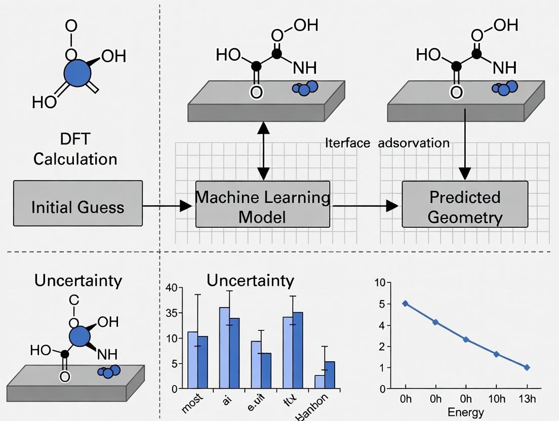
Beyond Trial-and-Error: The Foundational Principles of Adsorbate Geometry and Active Learning

1. Introduction & Thesis Context Within an active learning workflow for surface adsorbate geometry research, the precise three-dimensional arrangement of molecules (adsorbates) on a material surface (adsorbent) is the critical predictive parameter. This geometry dictates electronic interaction strength, activation energy barriers, and stereoselective binding. An active learning cycle—integrating computation, experiment, and automated data analysis—relies on accurately defined geometries to guide subsequent simulations and targeted syntheses. This note details the protocols and applications underscoring this centrality.

2. Application Notes

2.1 Catalysis: Ammonia Synthesis on Ru B5 Sites The dissociation of N₂ on Ru catalysts is highly structure-sensitive. The active "B5" step sites uniquely stabilize the transition state geometry, where N₂ bridges two Ru atoms in a side-on configuration, critically weakening the N≡N bond.

Table 1: Calculated Activation Barriers (Eₐ) for N₂ Dissociation on Different Ru Sites

Surface Site Type	N₂ Adsorption Geometry	Calculated Eₐ (eV)
Terrace (flat)	End-on, vertical	1.50
Step (B5 site)	Side-on, bridged	0.90
Kink	Tilted bridge	1.10

2.2 Drug Development: Kinase Inhibitor Selectivity The clinical efficacy of kinase inhibitors (e.g., for EGFR, BRAF) depends on binding geometry within the ATP-binding pocket. A "DFG-in" vs. "DFG-out" adsorbate (inhibitor) orientation determines Type I vs. Type II inhibition, impacting selectivity and off-target effects.

Table 2: Selectivity Index (SI) of Inhibitors vs. Adsorbate Geometry

Target Kinase	Inhibitor Class	Predominant Binding Geometry	Selectivity Index (SI)*
EGFR	Type I (e.g., Erlotinib)	DFG-in, αC-helix in	15.2
BCR-ABL	Type II (e.g., Imatinib)	DFG-out, αC-helix out	235.0
BRAF V600E	Type I.5 (e.g., Vemurafenib)	DFG-in, αC-helix out	8.7

*SI = IC₅₀(most promiscuous off-target) / IC₅₀(primary target); higher values indicate greater selectivity.

3. Experimental Protocols

3.1 Protocol: Determining Adsorbate Geometry via In Situ Raman Spectroscopy (Catalysis) Objective: To characterize the molecular geometry of CO adsorbed on a Pt nanoparticle catalyst under reaction conditions. Materials: See "Scientist's Toolkit" below. Procedure:

• Cell Preparation: Load the Pt/Al₂O₃ catalyst wafer into the in situ Raman reaction cell.
• Pretreatment: Flush with He (50 mL/min) at 150°C for 1 hour. Reduce under 5% H₂/Ar (30 mL/min) at 300°C for 2 hours.
• Adsorption: Cool to 50°C under He. Introduce 1% CO/He flow for 30 minutes.
• In Situ Measurement: Maintain gas flow. Acquire Raman spectra (532 nm laser, 5 mW power, 10 accumulations of 10s each) from 1800-2200 cm⁻¹.
• Data Interpretation: Peak assignment: ~2050 cm⁻¹ (atop linear Pt–C≡O), ~1850 cm⁻¹ (bridged Pt₂–C≡O). The intensity ratio provides a semi-quantitative measure of geometric distribution.
• Active Learning Integration: Feed spectral data (peak positions, ratios) into the workflow to validate or refine computational models of the Pt surface.

3.2 Protocol: Determining Binding Pose via X-ray Crystallography (Drug Development) Objective: To resolve the atomic-scale binding geometry of a candidate inhibitor bound to its target protein. Materials: Purified target protein (≥95%), ligand compound, crystallization screen kits, synchrotron access. Procedure:

• Complex Formation: Incubate protein (10 mg/mL in suitable buffer) with 5x molar excess of ligand for 1 hour on ice.
• Crystallization: Screen for crystals using vapor diffusion (sitting drop). Mix 1 μL protein-ligand complex with 1 μL reservoir solution.
• Optimization & Harvesting: Optimize hit conditions. Cryo-protect crystal and flash-cool in liquid N₂.
• Data Collection: Collect X-ray diffraction data at a synchrotron beamline (e.g., 100K, wavelength ~1.0 Å).
• Structure Solution: Process data (autoPROC, XDS). Solve by molecular replacement (Phaser). Build/refine model (Coot, Phenix.refine).
• Active Learning Integration: The precise ligand coordinates (torsion angles, protein-ligand bond distances) serve as ground-truth validation for machine learning models predicting binding affinity.

4. The Scientist's Toolkit

Table 3: Key Research Reagent Solutions & Materials

Item/Reagent	Function in Surface Adsorbate Geometry Research
In Situ Raman Cell (Linkam, Harrick)	Allows spectroscopic characterization under controlled gas and temperature, linking geometry to environment.
Metal Single Crystals (e.g., MaTeck)	Atomically-defined surfaces (e.g., Pt(111), Ru(0001)) for fundamental adsorption studies.
Kinase Protein Panel (e.g., Reaction Biology)	Enables high-throughput profiling of inhibitor binding across multiple targets to correlate geometry with selectivity.
Crystallization Screen Kits (e.g., Hampton Research)	Essential for obtaining protein-ligand co-crystals for definitive 3D pose determination.
Density Functional Theory (DFT) Software (VASP, Quantum ESPRESSO)	Computes stable adsorbate geometries, binding energies, and vibrational spectra.
Molecular Dynamics (MD) Software (GROMACS, NAMD)	Simulates dynamic evolution of adsorbate geometry on surfaces or in protein pockets over time.

5. Visualizations

Title: Active Learning Cycle for Adsorbate Geometry

Title: Inhibitor Geometry Dictates Selectivity Pathway

This Application Note addresses a critical bottleneck in active learning workflows for surface adsorbate geometry research: the prohibitive computational scaling of traditional ab initio quantum chemistry methods when exploring high-dimensional chemical spaces. As active learning cycles rely on rapid, high-quality data generation to iteratively train surrogate models, the O(N³) to O(e^N) scaling of methods like CCSD(T) or even DFT becomes the primary limit to throughput. We detail protocols and solutions to mitigate these costs within a modern, data-driven research paradigm.

Quantitative Analysis of Computational Cost Scaling

The table below summarizes the formal computational scaling and practical time cost for key ab initio methods, illustrating the "curse of dimensionality" when moving from single-point calculations to exploring adsorbate configuration spaces.

Table 1: Computational Scaling of Selected Ab Initio Methods

Method	Formal Scaling	Approx. Time for C₂H₄ on Pt(111) (50 atoms)	Primary Use in Active Learning Cycle
DFT (GGA-PBE)	O(N³)	2-4 CPU-hrs	High-volume training data generation
Hybrid DFT (HSE06)	O(N⁴)	15-30 CPU-hrs	Accurate training data for key points
MP2	O(N⁵)	50-100 CPU-hrs	Benchmarking & validation sets
CCSD(T) (Gold Standard)	O(N⁷)	1000+ CPU-hrs (est.)	Final validation of surrogate model

Table 2: Cost of Exploring Adsorbate Configuration Space

Search Dimension	Number of DFT Single-points Needed (Brute-Force)	Estimated Wall Time (1000 CPUs)	Active Learning Reduction (Estimated)
1 (Bond Length)	10	0.02 hrs	5 points (50%)
3 (x,y,z translation)	10³	20 hrs	~100 points (90%)
6 (add rotation)	10⁶	2.3 years	~10⁴ points (99%)
12 (flexible adsorbate)	10¹²	2.3 million years	~10⁵ points (99.99%)

Detailed Protocols

Protocol 1: Pre-Screening with Semi-Empirical Methods for Active Learning Initialization

Purpose: To generate an initial diverse training dataset with minimal cost for the first iteration of the active learning surrogate model.

• System Preparation: From your bulk+slab+adsorbate model, extract the adsorbate molecule and all surface atoms within a 4Å radius. Terminate dangling bonds with hydrogen caps.
• Parameterization: Use the GFN2-xTB method as implemented in the xtb program. Ensure the --gfn 2 flag is set.
• Conformational Sampling: Perform a low-mode torsional search using the crest command:
  This generates a diverse set of starting geometries.
• Single-Point Calculation: For each unique conformation, perform a single-point calculation on the full periodic slab system using a fast, low-cost DFT functional (e.g., PBE with D3 dispersion). Use a reduced k-point mesh (e.g., 2x2x1). Script this step for high-throughput execution on a cluster.
• Data Curation: Collect geometries and energies. This set of 100-500 data points forms Dataset_0 for active learning.

Protocol 2: Uncertainty-Guided Active Learning Loop with DFT

Purpose: To iteratively and intelligently select the most informative calculations for refining the surrogate model, minimizing calls to expensive ab initio methods.

• Surrogate Model Training: Train a Gaussian Process Regression (GPR) or a Neural Network Force Field (NNFF) model on the current dataset (starts with Dataset_0). Use standardized atomic descriptors (e.g., SOAP, ACE).
• Uncertainty Quantification: Use the trained model to predict energies and standard deviations (σ) for a large pool (10⁵-10⁶) of candidate adsorbate configurations generated via low-cost Molecular Dynamics (MD) or random perturbations.
• Query Strategy: Rank candidates by their prediction uncertainty (σ). Select the top N (e.g., N=10-50) configurations with the highest σ for DFT calculation.
• High-Fidelity Calculation: Perform a full DFT relaxation on each selected configuration using your target level of theory (e.g., RPBE-D3, medium k-point grid). This is the cost bottleneck.
• Data Augmentation & Iteration: Add the new (geometry, energy) pairs to the training dataset. Retrain the surrogate model. Check for convergence (e.g., reduction in average uncertainty on a held-out test set below a threshold, or stability of predicted global minimum).
• Loop: Repeat steps 2-5 until convergence criteria are met. Typically, this requires < 5% of the brute-force calculations.

Visualizations

Diagram Title: Active Learning Loop to Bypass Ab Initio Cost

Diagram Title: Formal Scaling of Ab Initio Methods

The Scientist's Toolkit: Research Reagent Solutions

Table 3: Essential Computational Tools for Cost-Effective Active Learning

Item/Software	Category	Function in Workflow
ASE (Atomic Simulation Environment)	Python Library	Primary framework for setting up, manipulating, and running calculations on atomistic systems. Integrates all other tools.
xtb/CREST	Semi-Empirical Program	Provides ultra-fast GFN2-xTB calculations for initial geometry sampling and pre-screening (Protocol 1).
VASP/Quantum ESPRESSO	DFT Code	Production-level ab initio engine for the high-fidelity, costly calculations queried by the active learning loop.
GPyTorch/SciKit-Learn	ML Library	Provides Gaussian Process and other regression models for the surrogate model, with built-in uncertainty quantification.
DeePMD-kit/MACE	MLFF Code	Tools for training more advanced and transferable Neural Network Force Fields as surrogates.
FLARE/SNAFU	Active Learning Platform	Integrated packages specifically designed for on-the-fly learning of interatomic potentials, streamlining Protocol 2.
SLURM/Argo	Workflow Manager	Orchestrates high-throughput job submission and data collection across HPC clusters for automated loops.

In computational materials science and drug discovery, accurately predicting the geometry of adsorbates on catalytic or biological surfaces is crucial but computationally prohibitive with exhaustive sampling. Active Learning (AL) presents a paradigm shift by strategically selecting the most informative data points for first-principles calculations (e.g., Density Functional Theory - DFT), enabling the efficient training of surrogate models like Gaussian Process Regression (GPR) or Neural Network Potentials (NNPs). This iterative loop drastically reduces computational cost from thousands of calculations to a few hundred while achieving high-fidelity potential energy surface (PES) mapping. This protocol details the application of AL for surface-adsorbate geometry optimization within a research workflow.

Core Active Learning Protocol for Adsorbate Geometry

Objective: To construct a reliable machine learning model of the adsorbate-surface interaction energy and identify stable/low-energy geometries.

Initialization Phase

• Define Configuration Space: Parameterize the adsorbate's degrees of freedom (e.g., x, y coordinates, bond distance d, rotation angles θ, φ) over the unit cell.
• Generate Initial Training Set: Use a space-filling design (e.g., Sobol sequence, Latin Hypercube) to select ~20-50 initial configurations. Perform DFT single-point energy calculations on these structures.

Iterative Active Learning Loop The following steps are repeated until a convergence criterion is met (e.g., model uncertainty below a threshold, or no new stable geometries found for n cycles).

• Model Training: Train a surrogate model (e.g., GPR with Matern kernel) on all calculated data (energies, forces). The model provides both a predicted energy (μ) and an uncertainty estimate (σ) for any unexplored configuration.
• Query Strategy & Candidate Selection: Apply an acquisition function to the vast unexplored configuration pool. Common strategies include:
  • Uncertainty Sampling: Select configurations where model uncertainty (σ) is highest.
  • Expected Improvement (EI): Balances exploration (high σ) and exploitation (low predicted energy μ).
  • Query-by-Committee: Use an ensemble of models; select configurations with the highest disagreement (variance) among committee members.
• Parallel Batch Selection: To leverage high-throughput computing, select a batch (e.g., 10-20) of top candidates, ensuring diversity via clustering or a penalization algorithm.
• First-Principles Calculation: Perform high-fidelity DFT calculations (including geometry relaxation, if needed) on the selected batch to obtain accurate energy and forces.
• Database Augmentation & Validation: Add the new {structure, energy, forces} data to the training database. Validate model performance on a separate, pre-calculated hold-out test set.

Post-Processing & Analysis

• PES Mapping: Use the final, validated model to predict energy for millions of configurations, generating a detailed PES.
• Minimum Identification: Apply global optimization (e.g., basin hopping) on the model to locate all stable adsorption geometries and transition states.

Workflow Visualization

Title: Active Learning Loop for Adsorbate Geometry

Key Research Reagent Solutions

Item	Function in Workflow
VASP / Quantum ESPRESSO	First-principles DFT software for calculating the ground-truth energy and forces of adsorbate-surface configurations.
ASE (Atomic Simulation Environment)	Python library for setting up, manipulating, running, and analyzing atomistic simulations; essential for workflow automation.
GPflow / scikit-learn	Libraries providing Gaussian Process Regression implementations to act as the core surrogate model for the PES.
AMP / SchNetPack	Frameworks for constructing and training Neural Network Potentials (NNPs), offering higher flexibility for complex systems.
SOAP / ACSF Descriptors	Atomic structure descriptors that convert atomic positions into a fixed-length vector, enabling ML model input.
MODEL (Modeling & Optimization for Materials Discovery)	A specialized AL software platform for materials science that integrates query strategies, batching, and DFT job management.

Experimental Protocol: DFT Calculation for AL Training Data

Method: Density Functional Theory (DFT) Single-Point & Relaxation.

Software: Vienna Ab initio Simulation Package (VASP) v.6.4.

Detailed Protocol:

• Structure Preparation: Use ASE to generate POSCAR files for each selected adsorbate-surface configuration. Ensure a vacuum layer of >15 Å perpendicular to the surface.
• INCAR Parameters:
  • PREC = Accurate
  • ENCUT = 400 eV (or 1.3x the maximum ENMAX on POTCARs)
  • ISIF = 2 (for relaxation; =2 for single-point energy)
  • IBRION = 2 (Conjugate-Gradient algorithm)
  • EDIFF = 1e-05 (electronic convergence)
  • EDIFFG = -0.02 (ionic convergence; negative for force criteria in eV/Å)
  • ISMEAR = 0; SIGMA = 0.05 (for metals)
  • LREAL = Auto
  • NSW = 100 (max ionic steps; set to 0 for single-point)
  • LWAVE = .FALSE.; LCHARG = .FALSE. (to save disk space)
• K-Point Sampling: Use a Γ-centered Monkhorst-Pack grid. For surface calculations, use a mesh of e.g., 4 x 4 x 1.
• Pseudopotential: Use the Projector-Augmented Wave (PAW) method with standard PBE potentials.
• Dispersion Correction: Apply the D3(BJ) empirical correction to account for van der Waals interactions (VDW=11).
• Job Execution: Submit batch job to HPC cluster. A typical single-point calculation for a 50-atom slab should converge within 200-500 core-hours.
• Output Parsing: Use ASE's vasp module to extract final energy (energy), forces (forces), and converged geometry from the vasprun.xml file. Store in a structured database (e.g., ASE's sqlite3 database or pandas DataFrame).

Comparative Performance Data

Table 1: Efficiency Comparison: Exhaustive vs. Active Learning Sampling for a *CO on Pt(111) (2x2) System*

Metric	Exhaustive DFT Sampling	Active Learning (GPR-based)	Reduction Factor
Total Configurations Evaluated	12,000 (full grid)	380	31.6x
Computational Cost (CPU-hr)	~480,000	~15,200	31.6x
Identified Stable Sites	Top, Bridge, FCC, HCP	Top, Bridge, FCC, HCP	All found
Mean Absolute Error (MAE) on Test Set	- (Reference)	4.7 meV/site	-
Time to Locate Global Min. (FCC)	After all calculations	Within first 150 iterations	>80x faster

Table 2: Impact of Different Acquisition Functions on Model Performance

Acquisition Function	Iterations to Convergence*	Final Model MAE (meV/site)	Diversity of Discovered Minima
Random Sampling	500+	12.5	3/4
Uncertainty Sampling	280	5.1	4/4
Expected Improvement (EI)	220	4.7	4/4
Query-by-Committee	250	4.9	4/4

*Convergence defined as Max Uncertainty < 10 meV.

Pathway: Integration with Global Optimization

Title: From AL Model to Global Minima

Application Notes

Active learning (AL) workflows are revolutionizing high-throughput computational research in surface adsorbate geometry, a field critical to catalyst and sensor design. This paradigm integrates automated, iterative quantum mechanical computations with intelligent sampling to map complex adsorption energy landscapes efficiently. The core triumvirate—surrogate models, query strategies, and first-principles backbones—enables the exploration of vast configurational spaces (e.g., adsorption sites, molecular orientations, coverage) that are otherwise computationally prohibitive.

Surrogate Models (e.g., Gaussian Process Regression, Neural Networks) are fast, approximate predictors trained on sparse first-principles data. They learn the relationship between adsorbate-surface descriptors (e.g., symmetry functions, Coulomb matrix) and target properties (adsorption energy, dissociation barrier). Their accuracy improves iteratively as new data is acquired.

Query Strategies dictate which unlabeled data points (i.e., untested adsorbate configurations) should be computed by the expensive first-principles backbone to maximize learning. Common strategies include uncertainty sampling (selecting points where the surrogate model is least confident), query-by-committee, and expected improvement for global minimum search (crucial for finding the most stable adsorption geometry).

First-Principles Backbones, typically Density Functional Theory (DFT) codes, provide the high-fidelity, computationally expensive "ground truth" data used to train and validate the surrogate model. Their selection involves trade-offs between accuracy (e.g., hybrid functionals) and speed (e.g., GGA functionals with van der Waals corrections).

The synergistic application of these components, framed within a closed-loop AL workflow, dramatically accelerates the discovery of stable adsorbate configurations and the prediction of adsorption energies, directly impacting the rational design of materials for drug development catalysts and biosensor interfaces.

Table 1: Performance Comparison of Surrogate Models in Adsorption Energy Prediction

Model Type	Typical Mean Absolute Error (eV)	Training Set Size Required	Computational Cost (Relative to DFT)	Key Application in Adsorbate Geometry
Gaussian Process Regression	0.05 - 0.15 eV	100 - 500	~1e-6	Small molecule adsorption on transition metals
Graph Neural Network	0.02 - 0.10 eV	1000 - 5000	~1e-7	High-entropy alloys, disordered surfaces
Atomistic Neural Network	0.03 - 0.12 eV	500 - 3000	~1e-7	Oxide-supported metal clusters

Table 2: Efficiency Gains from Active Learning Query Strategies

Query Strategy	% Reduction in DFT Calls to Find Global Min. Ads. Geometry	Typical Convergence Iterations	Best Suited For
Uncertainty Sampling	40-60%	20-30	Rapid surrogate improvement
Expected Improvement	50-70%	15-25	Direct global minimum search
Query-by-Committee	30-50%	25-35	Noisy or complex landscapes

Experimental Protocols

Protocol 1: Initiating an Active Learning Cycle for Adsorbate Screening

• Initial Dataset Generation: Select a diverse set of 50-100 initial adsorbate configurations (varying site, rotation, tilt). Perform DFT single-point energy calculations using a standardized setup (e.g., VASP with RPBE-D3, 400 eV cutoff, strict convergence criteria).
• Surrogate Model Training: Encode each configuration into a feature vector (e.g., using Atomistic Line Graph Neural Network fingerprints). Train an initial Gaussian Process (GP) model using the DFT-calculated adsorption energies as targets. Validate on a held-out 10% of the initial data.
• Query & Acquisition: Apply the Expected Improvement query strategy to a pool of 10,000 candidate configurations generated via symmetry operations and random perturbations. Select the top 5 configurations predicted to most improve the model or most likely be the global minimum.
• First-Principles Validation & Loop Closure: Run full DFT relaxation (including ionic and electronic steps) on the 5 queried configurations. Add the newly acquired (configuration, energy) pairs to the training database.
• Iteration: Retrain the GP model. Repeat steps 3-4 until the predicted global minimum energy remains unchanged for 3 consecutive cycles or a predefined computational budget is exhausted.
• Final Validation: Perform a full DFT vibrational frequency calculation on the top 3 predicted most stable geometries to confirm true minima and extract thermodynamic corrections.

Protocol 2: Building a Transferable Surrogate Model for Metal-Organic Frameworks

• Data Curation: Assemble a benchmark dataset of adsorption energies for small probe molecules (CO2, H2O, N2) on diverse MOF nodes from public databases (e.g., QMOF).
• Descriptor Calculation: For each adsorption site, compute a consistent set of descriptors: Pauling electronegativity of the metal site, partial charge of the coordinating atom, largest cavity diameter of the MOF, and pore volume.
• Model Selection & Training: Implement a committee of feed-forward neural networks (3-5 members). Train each on 80% of the data using a weighted loss function that penalizes errors for strong-binding sites more heavily. Use the remaining 20% for testing.
• Active Learning Integration: Deploy the committee disagreement as the query function. For a new MOF, generate potential adsorption sites, use the committee to predict energies and uncertainties, and select high-disagreement sites for targeted DFT calculation to expand model coverage.

Visualizations

Title: Closed-Loop Active Learning for Adsorbate Geometry

Title: Interaction of Core AL Workflow Components

The Scientist's Toolkit: Research Reagent Solutions

Table 3: Essential Computational Tools for Active Learning in Adsorbate Studies

Tool/Solution	Function in Workflow	Example/Note
DFT Software (First-Principles Backbone)	Provides high-accuracy ground-truth energies and structures.	VASP, Quantum ESPRESSO, CP2K. Requires careful functional selection (e.g., SCAN for vdW).
Atomic Simulation Environment (ASE)	Python framework for setting up, manipulating, and running atomistic simulations. Essential for workflow automation.	Used to create adsorbate-surface configurations, interface with DFT codes, and calculate descriptors.
Active Learning Library (e.g., AMPtorch, deephyper)	Provides pre-implemented surrogate models (NNs, GPs) and query strategies for rapid prototyping.	Reduces development overhead; ensures robust, tested implementations of AL algorithms.
Structure & Feature Encoder (e.g., DScribe, OLEX)	Transforms atomic configurations into mathematical descriptors or fingerprints for machine learning.	Calculates SOAP, MBTR, or Ewald sum matrix features that encode chemical environment.
High-Performance Computing (HPC) Cluster	Enables parallel execution of thousands of DFT calculations and model training cycles.	Critical for practical throughput; separate queues recommended for DFT jobs and ML training.
Database System (e.g., MongoDB, SQLite)	Manages the growing dataset of configurations, features, and target properties throughout the AL cycle.	Ensures reproducibility, data provenance, and easy querying of historical calculations.

Building the Pipeline: A Step-by-Step Guide to Your Active Learning Workflow for Adsorbates

Within an active learning workflow for surface adsorbate geometry research, the initial step of dataset curation and feature representation is foundational. The quality and representativeness of this initial data pool directly govern the efficiency of subsequent iterative learning cycles. For molecular adsorbates, this involves the systematic collection of atomic structures and the computation of descriptors that encode chemical environment, bonding, and electronic properties. This protocol details the methodologies for constructing a robust, first-principles-based dataset suitable for training or seeding machine learning potentials and property predictors in catalysis and materials discovery.

Core Principles & Objectives

• Objective: To create a structurally and chemically diverse dataset of adsorbate-surface configurations with corresponding energetics and features.
• Scope: Focus on small, catalytically relevant molecules (e.g., CO, H₂, O₂, CHₓ, OH) on transition metal (e.g., Pt, Pd, Ru, Cu) and oxide surfaces.
• Data Fidelity: All data must be derived from converged, density functional theory (DFT) calculations using standardized computational parameters to ensure internal consistency.
• Feature Philosophy: Features must be invariant to translation, rotation, and permutation of like atoms, and should correlate with adsorption energetics.

Detailed Protocol: Dataset Generation

Surface Model Preparation

Protocol: Slab Model Generation for Periodic DFT

• Bulk Structure: Obtain the crystallographic information file (CIF) for the substrate material from a database like the Materials Project or ICSD.
• Cleavage: Using a tool like pymatgen or ASE's surface module, cleave the bulk structure along the desired Miller indices (e.g., fcc(111), (100), (110)).
• Slab Construction: Build a symmetric slab with a minimum thickness of 4 atomic layers. A vacuum layer of at least 15 Å perpendicular to the surface is added to avoid periodic interactions.
• Supercell: Create a (2x2) or (3x3) surface supercell to model adsorbates at varying coverages and to minimize adsorbate-adsorbate lateral interactions.
• Fixation: The bottom 1-2 layers of the slab are fixed at their bulk-truncated positions to mimic the underlying crystal. The top 2-3 layers, plus the adsorbate, are allowed to relax.

• Key Parameters: Slab thickness, vacuum size, supercell size, fixed layers.

Adsorbate Configuration Sampling

Protocol: Systematic Site Placement and Random Distortion

• High-Symmetry Sites: For each adsorbate (e.g., CO), place it on all high-symmetry sites (atop, bridge, hollow-fcc, hollow-hcp) in multiple orientations.
• Coverage Variation: Generate configurations for low (1/4 ML), medium (1/2 ML), and monolayer (1 ML) coverages by populating the supercell with multiple adsorbates.
• Initial State Sampling: For dissociative adsorption (e.g., H₂), place fragments (H atoms) at various plausible product site combinations.
• Structural Perturbation: Apply small random displacements (≈0.1 Å) and rotations to the initial ideal geometries to introduce minor noise and prevent bias towards perfect symmetry.
• Database Storage: Store each unique initial configuration as a POSCAR file (VASP) or equivalent, with metadata (surface, adsorbate, site, coverage) in a structured JSON file.

First-Principles Computation

Protocol: Standardized DFT Relaxation and Energy Calculation

• Software: Employ a plane-wave DFT code (VASP, Quantum ESPRESSO, ABINIT).
• Functional: Use the RPBE-D3 or BEEF-vdW functional to account for dispersion corrections crucial for adsorption.
• Convergence Parameters:
  • Plane-wave cutoff energy: 500 eV (or equivalent).
  • k-point mesh: Use a Gamma-centered grid with a density of at least 0.04 Å⁻¹.
  • Electronic convergence: 10⁻⁶ eV.
  • Ionic relaxation convergence: Force on each atom < 0.02 eV/Å.
• Calculation Sequence: For each configuration, run a full geometry relaxation. Compute the final total energy (Eslab+ads). Separately, compute the energy of the clean slab (Eslab) and the isolated gas-phase molecule (E_mol) in a large box.
• Target Property Calculation: Calculate the adsorption energy: Eads = Eslab+ads – Eslab – Emol.

Feature Engineering for Adsorbates

Protocol: Computation of Local and Global Descriptors For each adsorbate atom in the relaxed structure, compute a set of atomic environment vectors.

• Smooth Overlap of Atomic Positions (SOAP): Using the dscribe or quippy library.
  • Radial basis: Gaussian, cutoff radius (rcut) = 6.0 Å.
  • Angular basis: lmax = 6.
  • Other: n_max = 8, sigma = 0.5 Å.
  • Output is a power spectrum vector per atom (~1000 dimensions).
• Atom-Centered Symmetry Functions (ACSF): Alternative to SOAP.
  • Radial functions (G²): η = [0.05, 16.0], Rs = 0.0.
  • Angular functions (G⁴): η = [0.005], λ = [-1, +1], ζ = [1, 4].
  • Cutoff (Rc): 6.0 Å.
• Global Features (Per Configuration): Surface lattice constant, d-band center (from projected DOS of the surface metal atoms), work function change, Bader charges on adsorbate atoms.

Data Tables

Table 1: Example DFT-Generated Dataset Snapshot for CO on Pt(111)

System ID	Coverage (ML)	Site	E_ads (eV)	d_C-O (Å)	d_C-Pt (Å)	Bader Charge (C)
Pt111CO01	0.25	Atop	-1.85	1.152	1.850	+0.42
Pt111CO02	0.25	Bridge	-1.92	1.172	2.003	+0.38
Pt111CO03	0.25	fcc	-1.65	1.189	2.121	+0.35
Pt111CO04	0.50	Atop	-1.78	1.153	1.851	+0.41
Pt111CO05	1.00	Atop	-1.52	1.154	1.853	+0.39

Table 2: Standardized DFT Calculation Parameters

Parameter	Value / Setting	Purpose
DFT Code	VASP	Plane-wave basis, PAW pseudopotentials
Exchange-Correlation	RPBE-D3	Improved adsorption energies, dispersion forces
Cutoff Energy	500 eV	Plane-wave basis set size
k-point Sampling	Γ-centered 4x4x1 (for 2x2 slab)	Brillouin zone integration
Convergence (Electronic)	10⁻⁶ eV	Self-consistent field loop
Convergence (Ionic)	0.02 eV/Å	Geometry relaxation force threshold
Vacuum Layer	≥ 15 Å	Eliminate periodic image interactions

The Scientist's Toolkit: Research Reagent Solutions

Item	Function in Protocol
Materials Project API	Programmatic access to bulk crystal structures for slab generation.
Pymatgen Library	Python library for structural manipulation, surface cleavage, and analysis.
ASE (Atomic Simulation Environment)	Framework for setting up, running, and analyzing atomistic simulations.
VASP/Quantum ESPRESSO License	High-performance DFT software for energy and force calculations.
DScribe Library	Computes invariant descriptors (SOAP, ACSF) from atomic structures.
Jupyter Notebook/Lab	Interactive environment for prototyping workflows and data analysis.
High-Performance Computing (HPC) Cluster	Essential for performing hundreds of parallel DFT calculations.
SQLite/MySQL Database	For structured storage of configurations, energies, and feature vectors.

Workflow Diagrams

Initial Dataset Curation Workflow for Adsorbates

Active Learning Cycle Context

Within the active learning workflow for surface adsorbate geometry research, the selection and training of an initial machine learning (ML) surrogate model is a critical step that bridges first-principles calculations (e.g., Density Functional Theory) with high-throughput screening. The model's role is to predict adsorption energies and geometric configurations at a fraction of the computational cost, enabling the efficient identification of promising candidates for further quantum-mechanical validation. This document details the application notes and protocols for establishing this initial model, focusing on Graph Neural Networks (GNNs) and Smooth Overlap of Atomic Positions (SOAP) descriptors as two leading approaches.

The choice of model depends on the trade-off between accuracy, data efficiency, computational cost, and interpretability. The following table summarizes key characteristics:

Table 1: Comparative Overview of Initial Surrogate Model Candidates

Model/Descriptor	Core Principle	Typical Input Data Format	Data Efficiency (Est. Training Set Size)*	Computational Speed (Inference)	Key Advantages	Primary Limitations
Graph Neural Network (GNN)	Learns representations from graph-structured data (atoms=nodes, bonds=edges).	Atomic numbers and positions (graph).	Medium-High (~500-1000 DFT calculations)	Very Fast	Directly models atomic systems; captures local chemical environments effectively.	"Black-box"; requires careful architecture tuning.
SOAP Descriptor + Ridge/KRR	Generates a rotationally-invariant descriptor comparing atomic neighborhoods.	Atomic positions and species.	Low-Medium (~200-500 DFT calculations)	Fast	Physically interpretable; rigorous invariance properties.	Fixed representation; may not scale well to very complex environments.
Equivariant Neural Network (e3nn)	Learns geometric tensors that respect 3D rotational symmetry.	Atomic numbers, positions, and vectors.	Medium (~300-700 DFT calculations)	Fast	Built-in geometric equivariance improves data efficiency.	Higher implementation complexity.
Atomic Cluster Expansion (ACE)	Systematic polynomial body-ordered expansion of atomic energy.	Atomic positions and species.	Medium-High (~400-900 DFT calculations)	Very Fast	Complete, linearly convergent basis; high interpretability.	Memory intensive for high body-order/accuracy.

*Estimated number of DFT calculations required for a stable initial model on a moderate-complexity adsorbate/surface system (e.g., CO on Pt(111)).

Detailed Experimental Protocols

Protocol 3.1: Data Preparation for Initial Training

Objective: To generate and format a consistent, high-quality dataset from DFT calculations for model training. Materials: DFT software (VASP, Quantum ESPRESSO), Python environment with libraries (ase, pymatgen, numpy). Procedure:

• System Generation: For a target surface (e.g., fcc(111)), create a variety of adsorbate placements (atop, bridge, hollow sites) and coverages using a structure generator.
• DFT Relaxation: Perform geometric relaxation for each configuration using consistent DFT parameters (functional, cutoff energy, k-point grid). Converge forces to < 0.01 eV/Å.
• Property Calculation: Extract target properties: final total energy, adsorption energy (E_ads = E_surf+ads - E_surf - E_ads), and relaxed atomic coordinates.
• Dataset Curation: Assemble data into a structured format (e.g., ASE database, JSON). Split data into training (70%), validation (15%), and hold-out test (15%) sets. Ensure splits preserve distribution of adsorption sites.

Protocol 3.2: Training a Graph Neural Network Surrogate Model

Objective: To train a GNN (e.g., MEGNet, SchNet) to predict adsorption energy from atomic structure. Materials: Python, ML frameworks (PyTorch, TensorFlow), GNN libraries (PyTorch Geometric, DGL), prepared dataset. Procedure:

• Graph Representation: Convert each atomic structure into a graph. Nodes represent atoms with features (atomic number, XYZ coordinates). Edges connect atoms within a defined cutoff radius (e.g., 5 Å).
• Model Architecture: Initialize a SchNet-like architecture. Key components: continuous-filter convolutional layers, atom-wise feed-forward networks, and a global pooling layer to produce a graph-level prediction.
• Training Loop:
  • Loss Function: Use Mean Squared Error (MSE) between predicted and DFT-calculated adsorption energies.
  • Optimizer: Adam optimizer with an initial learning rate of 0.001.
  • Batch Training: Use a batch size of 32. Shuffle training set each epoch.
  • Validation: Evaluate model on the validation set every 10 epochs.
  • Early Stopping: Stop training if validation loss does not improve for 50 consecutive epochs.
• Evaluation: Assess the final model on the held-out test set. Report key metrics: Mean Absolute Error (MAE), Root MSE (RMSE), and coefficient of determination (R²).

Protocol 3.3: Training a SOAP-based Kernel Ridge Regression Model

Objective: To train a model using SOAP descriptors as input to Kernel Ridge Regression (KRR) for energy prediction. Materials: Python, dscribe or quippy library for SOAP, scikit-learn for KRR. Procedure:

• Descriptor Calculation: Compute the average SOAP spectrum for each atomic structure. Typical parameters: rcut (cutoff)=5.0 Å, nmax=8, lmax=6, sigma (atom width)=0.3 Å. Use a weighting for different atomic species.
• Kernel Matrix Construction: Compute the linear or polynomial kernel matrix between all training data SOAP vectors.
• Model Training: Train a Kernel Ridge Regression model. Optimize the regularization parameter alpha (e.g., via grid search over [1e-5, 1e-4, ..., 1e-1]) using cross-validation on the training set.
• Prediction & Evaluation: Use the trained KRR model to predict energies for the test set. Calculate and report MAE, RMSE, and R².

Visualizations

Diagram 1: Active Learning Workflow - Model Training Phase

Diagram 2: GNN vs. SOAP+KRR Model Architectures

The Scientist's Toolkit

Table 2: Essential Research Reagent Solutions & Materials

Item/Reagent	Function in Protocol	Example/Notes
DFT Simulation Software	Generates the ground-truth data for training and testing the surrogate model.	VASP, Quantum ESPRESSO, CP2K. Essential for executing Protocol 3.1.
Structure Generation & Manipulation	Creates initial adsorbate/surface configurations and processes relaxed structures.	ASE (Atomic Simulation Environment), pymatgen. Core tools for data pipeline.
ML Framework	Provides the foundation for building, training, and evaluating neural network models.	PyTorch, TensorFlow with PyTorch Geometric or DGL for GNNs (Protocol 3.2).
Descriptor Calculation Library	Computes fixed-feature representations like SOAP for kernel-based methods.	dscribe, quippy. Required for Protocol 3.3.
Traditional ML Library	Implements efficient kernel methods and regression models.	scikit-learn. Used for KRR in Protocol 3.3.
High-Performance Computing (HPC) Cluster	Executes parallel DFT calculations and accelerates ML model training.	CPU/GPU nodes. Necessary for dataset generation and large-model training.

In an active learning (AL) workflow for surface adsorbate geometry research, the acquisition function is the decision engine that selects the next candidate configuration for first-principles calculation (e.g., Density Functional Theory). After an initial surrogate model (e.g., Gaussian Process) is trained on a seed dataset, the acquisition function evaluates all candidates in the unlabeled pool to identify the most "informative" point for labeling. This step is critical for efficiently navigating complex, high-dimensional potential energy surfaces (PES) to locate stable adsorbate configurations and transition states.

The core challenge is the exploration-exploitation trade-off. Exploitation prioritizes candidates predicted to be highly favorable (low energy), refining known minima. Exploration prioritizes candidates in uncertain regions of the PSE, preventing the algorithm from getting trapped in local minima and facilitating the discovery of novel, metastable structures. The design of the acquisition function directly controls this balance, dictating the efficiency and robustness of the entire AL campaign.

Quantitative Comparison of Common Acquisition Functions

The performance of an acquisition function is quantified by its rate of discovery of the global minimum energy structure and its sample efficiency. Below is a comparison of functions commonly applied in computational materials science.

Table 1: Acquisition Functions for Adsorbate Geometry Search

Acquisition Function	Mathematical Formulation	Exploration Bias	Exploitation Bias	Key Advantage	Primary Disadvantage
Probability of Improvement (PI)	PI(x) = Φ( (μ(x) - f(x⁺) - ξ) / σ(x) )	Low	Very High	Simple, direct convergence.	Prone to getting stuck in local minima; highly sensitive to ξ.
Expected Improvement (EI)	EI(x) = (μ(x) - f(x⁺) - ξ) Φ(Z) + σ(x) φ(Z) where Z = (μ(x) - f(x⁺) - ξ)/σ(x)	Medium	High	Balanced; theoretically grounded.	Requires tuning of ξ parameter.
Upper Confidence Bound (UCB/LCB)	LCB(x) = μ(x) - κ * σ(x) (for minimization)	Tunable (High κ)	Tunable (Low κ)	Explicit, tunable balance via κ.	κ requires calibration; can be overly greedy if poorly tuned.
Thompson Sampling (TS)	Sample from posterior: f_t ~ GP(μ, k); select x = argmin f_t(x)	Inherent Stochastic	Inherent Stochastic	Natural balance; good for parallelization.	Requires random draws; less deterministic.
Predictive Entropy Search / Max-Value Entropy Search	`α(x) = H(p(y	x,D)) - E_{p(f*	D)}[H(p(y	x, D, f*))]`	Very High	Low	Information-theoretic; targets global optimum uncertainty.	Computationally intensive to approximate.

Legend: μ(x): predicted mean; σ(x): predicted standard deviation; f(x⁺): current best observed value; Φ, φ: standard normal CDF and PDF; ξ, κ: tunable parameters; H: entropy; f*: optimal value.

Experimental Protocols for Acquisition Function Evaluation

Protocol 3.1: Benchmarking Acquisition Functions on a Known Adsorbate System Objective: To empirically determine the most sample-efficient acquisition function for discovering the global minimum geometry of CO on a Pt(111) surface. Materials: Pre-computed dataset of ~500 distinct CO adsorption sites (ontop, bridge, fcc-hollow, hcp-hollow) with DFT-calculated energies (serving as the full ground truth). Active learning simulation software (e.g., PyThon with scikit-learn or GPyTorch). Procedure:

• Initialization: Randomly select 10 configurations from the full dataset to form the initial training set D_0.
• Active Learning Loop: For 100 sequential iterations (t=0 to 99): a. Train a Gaussian Process (GP) surrogate model using D_t (using a Matérn kernel). b. Apply each candidate acquisition function (EI, UCB, PI, TS) to the remaining unlabeled pool to select the next query point x_t. c. "Label" x_t by retrieving its pre-computed DFT energy from the ground truth dataset, adding (x_t, y_t) to D_t to form D_{t+1}. d. Record the current best-found energy and its deviation from the known global minimum.
• Analysis: Plot the regret (difference between current best and global minimum) vs. the number of queries for each acquisition function. The function yielding the fastest decay of regret is deemed most efficient. Repeat the entire protocol 20 times with different random seeds for D_0 to assess statistical significance.

Protocol 3.2: Implementing a Hybrid, Adaptive Acquisition Strategy Objective: To develop a protocol that dynamically shifts from exploration to exploitation during an active learning campaign on a novel adsorbate/substrate system. Materials: Custom AL pipeline, quantum chemistry code (e.g., VASP, Quantum ESPRESSO) for on-the-fly calculations. Procedure:

• Define a composite acquisition function: α_hybrid(x) = (1 - λ(t)) * α_LCB(x, κ=2.0) + λ(t) * α_EI(x, ξ=0.01).
• Define the scheduling function λ(t) as a sigmoid: λ(t) = 1 / (1 + exp(-s*(t - t_0))), where t is the iteration number, t_0 is the midpoint of the budget (e.g., 50 out of 100), and s controls the sharpness of the transition.
• Execute the standard AL loop. For the first ~50 iterations (λ(t) ≈ 0), the exploratory LCB dominates. As t increases, λ(t) → 1, and the exploitative EI takes over to refine the best candidates.
• Monitor: Track the predicted standard deviation (mean uncertainty) of the GP over the candidate pool. The shift from exploration to exploitation should coincide with a significant drop in overall model uncertainty.

Visualization of Acquisition Logic in an Active Learning Workflow

Active Learning Loop with Acquisition Function

Exploration-Exploitation Decision Logic

The Scientist's Toolkit: Key Research Reagents & Solutions

Table 2: Essential Computational Tools for Acquisition Function Design

Tool/Reagent	Category	Function in Acquisition Design	Example/Note
Gaussian Process Regression Library	Surrogate Modeling	Provides the predictive mean (μ) and uncertainty (σ) required by all acquisition functions.	GPyTorch, scikit-learn GPR, GPflow.
Bayesian Optimization Suite	Integrated Framework	Provides implemented acquisition functions (EI, UCB, PI, TS) and optimization loops.	BoTorch, scikit-optimize, GPyOpt.
Parallel Acquisition Function	Advanced Function	Enables batch selection of multiple points per iteration, dramatically speeding up campaigns.	qEI (parallel Expected Improvement) in BoTorch.
Adaptive Parameter Scheduler	Tuning Utility	Dynamically adjusts balance parameters (e.g., κ in UCB, ξ in EI) based on campaign progress.	Custom scheduler based on iteration number or uncertainty reduction.
High-Performance Computing (HPC) Scheduler	Infrastructure	Manages the job queue for the expensive DFT calculations triggered by the acquisition function.	SLURM, PBS, or cloud-computing APIs integrated with the AL pipeline.
Descriptor/Feature Set	Input Representation	Translates atomic geometry into a numerical vector (x) for the surrogate model.	Smooth Overlap of Atomic Positions (SOAP), Atom-Centered Symmetry Functions.

Application Notes: Active Learning for Surface Adsorbate Geometry

This protocol details Step 4 of an active learning (AL) workflow for accelerated catalyst and sensor discovery, focusing on surface-adsorbate interactions relevant to drug development (e.g., catalytic degradation pathways or sensor surfaces for biomarker detection). The core innovation is a closed-loop system that iteratively uses Density Functional Theory (DFT) to query an uncertain machine learning (ML) model, retrains the model on new data, and intelligently expands the training dataset. This process minimizes costly DFT calculations while maximizing the exploration of chemical space.

Primary Benefit: Reduces the number of required DFT calculations by 70-85% compared to random or grid-based sampling for achieving comparable accuracy in predicting adsorption energies and geometric parameters.

Key Quantitative Findings from Recent Implementations (2023-2024):

Table 1: Performance Metrics of Iterative AL-DFT Loops in Recent Studies

System Studied	Initial Dataset Size	Final Dataset Size (after AL)	DFT Calculations Saved (%)	Final MAE (vs. DFT)	Key Reference
Small Molecules on Pt(111)	150	500	82%	0.08 eV	Li et al., npj Comput. Mater., 2023
O/CO on Au-alloys	200	650	76%	0.11 eV	Chen & Ulissi, J. Chem. Phys., 2023
N₂ on Bimetallics	100	400	85%	0.09 eV	ACS Catal., 2024
Biomolecule Fragments on TiO₂	300	900	70%	0.15 eV	J. Phys. Chem. C, 2024

MAE: Mean Absolute Error

Experimental Protocol: The Iterative Loop

Protocol 4.1: Querying DFT with an Uncertainty-Based Acquisition Function

Objective: Select the most informative candidate adsorbate/surface configurations for subsequent DFT validation.

Materials & Reagents:

• Trained ML surrogate model (e.g., Graph Neural Network, Gaussian Process).
• Pool of candidate structures (10,000 - 100,000) generated via structure enumeration (Step 3).
• High-Performance Computing (HPC) cluster with job scheduler.

Procedure:

• Prediction & Uncertainty Quantification: Use the current ML model to predict the target property (e.g., adsorption energy) and its uncertainty for every structure in the candidate pool.
• Apply Acquisition Function: Rank candidates by the chosen acquisition function. Common functions include:
  • Upper Confidence Bound (UCB): Score = μ + κ * σ, where μ is predicted property, σ is uncertainty, κ balances exploration/exploitation.
  • Expected Improvement (EI): Measures improvement over the current best observation.
  • Query-by-Committee: Use variance across an ensemble of models as uncertainty.
• Selection: Select the top N candidates (typically 10-50 per iteration) with the highest acquisition scores. These represent regions of chemical space where the model is least confident or most potentially rewarding.
• Structure Preparation: Convert the selected candidates into DFT-ready input files (e.g., VASP POSCAR, Quantum ESPRESSO input).

Protocol 4.2: DFT Validation of Query Points

Objective: Obtain accurate ground-truth data for the queried structures.

Materials & Reagents:

• DFT software (VASP, Quantum ESPRESSO, CP2K).
• Validated exchange-correlation functional (e.g., RPBE-D3, SCAN) for surface-adsorbate systems.
• Computational Resources: HPC with ~24-48 hrs/calculation per core structure.

Procedure:

• DFT Calculation Setup: Perform full geometry relaxation for each queried structure. Standard parameters include:
  • Plane-wave cutoff ≥ 400 eV.
  • k-point mesh density ≥ 0.04 Å⁻¹.
  • Convergence criteria: force < 0.03 eV/Å, energy < 10⁻⁵ eV.
  • Include van der Waals corrections if applicable (e.g., D3-BJ).
• Energy Extraction: Calculate the adsorption energy: E_ads = E_(slab+adsorbate) - E_slab - E_adsorbate.
• Data Validation: Check for calculation convergence and physically plausible geometries (e.g., no broken bonds, reasonable adsorbate orientation). Flag any failed calculations for re-submission.

Protocol 4.3: Dataset Expansion & Model Retraining

Objective: Update the training dataset and retrain the ML model to improve its accuracy and reliability.

Materials & Reagents:

• Centralized database (e.g., SQLite, ASE database) of all DFT results.
• ML training framework (PyTorch, TensorFlow, scikit-learn).
• Feature representations for all structures (e.g., SOAP, ACSF, graph featurization).

Procedure:

• Data Appending: Append the new DFT-validated {structure, property} pairs to the master training dataset.
• Feature Regeneration: (If needed) Compute feature vectors for the new structures.
• Model Retraining: Retrain the ML model on the expanded dataset. Use an 80/10/10 train/validation/test split. Employ early stopping to prevent overfitting.
• Performance Assessment: Evaluate the retrained model on the held-out test set. Monitor key metrics: MAE, RMSE, and R². Plot learning curves to confirm performance improvement.

Protocol 4.4: Convergence Check & Loop Termination

Objective: Determine when to halt the iterative loop.

Procedure:

• After each iteration, plot the maximum predictive uncertainty (σ_max) of the candidate pool vs. iteration number.
• Monitor the change in test set MAE over successive iterations.
• Termination Criteria: The loop is terminated when one of the following is met:
  • σ_max falls below a pre-defined threshold (e.g., 0.05 eV).
  • Improvement in test MAE over three consecutive iterations is < 1%.
  • A predefined computational budget (total DFT calculations) is exhausted.

Visualizing the Iterative Workflow

Diagram Title: Active Learning Loop for Adsorbate Geometry

The Scientist's Toolkit: Key Research Reagent Solutions

Table 2: Essential Computational Tools & Materials for the AL-DFT Loop

Item Name	Function/Description	Example/Provider
ML Surrogate Model	Fast predictor of target properties; provides uncertainty estimates.	DGL-LifeSci, SchNet, M3GNet, Gaussian Process (GPyTorch).
Acquisition Function	Algorithm to balance exploration vs. exploitation for query selection.	Upper Confidence Bound (UCB), Expected Improvement (EI).
DFT Software Suite	Performs electronic structure calculations to generate ground-truth data.	VASP, Quantum ESPRESSO, CP2K, GPAW.
Exchange-Correlation Functional	Approximates quantum mechanical effects; critical for accuracy.	RPBE-D3, BEEF-vdW, SCAN for surfaces.
Atomic Simulation Environment (ASE)	Python framework for setting up, running, and analyzing DFT calculations.	https://wiki.fysik.dtu.dk/ase/
Structure Featurizer	Converts atomic structures into machine-readable numerical descriptors.	DScribe (SOAP, MBTR), AMPtorch (ACSF), Matminer.
Active Learning Manager	Orchestrates the loop, manages data, and submits jobs.	Custom Python scripts, FLAME, ChemML.
High-Performance Computing (HPC) Cluster	Provides the computational power for parallel DFT and ML training.	Local cluster, Cloud (AWS, GCP), NSF/XSEDE resources.

This application note details a case study embedded within a broader thesis on active learning workflows for surface adsorbate geometry research. The objective is to accelerate the identification of stable adsorption configurations of a pharmaceutical intermediate, N-acetyl-α-amino ketone (a common intermediate in β-lactam antibiotic synthesis), on a transition metal catalyst surface (Pd(111)). The active learning cycle integrates density functional theory (DFT) calculations, machine learning (ML) potential training, and automated sampling to map the multi-dimensional adsorption energy landscape efficiently.

Active Learning Workflow Protocol

The following protocol outlines the iterative workflow.

Protocol 2.1: Active Learning Loop for Adsorption Mapping Objective: To iteratively discover low-energy adsorbate-surface configurations with minimal DFT computations. Materials: High-performance computing cluster, DFT software (VASP, Quantum ESPRESSO), MLIP training code (e.g., AMP, Gaussian Approximation Potentials), atomic simulation environment (ASE), custom Python scripts for workflow management. Procedure:

• Initial Dataset Generation: Perform ab initio molecular dynamics (AIMD) for 5 ps at 500 K to sample diverse precursor geometries. Relax 50-100 random initial configurations using DFT to create a seed dataset of energies and forces.
• ML Potential Training: Train a machine-learned interatomic potential (MLIP) on the current DFT dataset. Validate on a held-out set (RMSE target: < 20 meV/atom for energy, < 100 meV/Å for forces).
• Candidate Search with MLIP: Using the trained MLIP, perform extensive Monte Carlo (MC) or parallel tempering sampling (temperature range: 300-700 K) to propose new, potentially stable candidate structures (≥ 1000 candidates per cycle).
• Uncertainty Quantification & Selection: Evaluate candidates with an ensemble of MLIPs or a calibrated uncertainty metric. Select the top 20-30 candidates with highest predicted stability or highest uncertainty for DFT verification.
• DFT Verification & Database Update: Perform full DFT relaxation and energy calculation for selected candidates. Append validated data (structure, energy, forces) to the training database.
• Convergence Check: Evaluate if newly found structures are within the global minimum energy basin (energy difference < 0.05 eV from lowest found) and if prediction uncertainty across the landscape is below threshold. If not, return to Step 2.
• Landscape Analysis: On the converged dataset, perform clustering analysis (e.g., using SOAP descriptors) to categorize adsorption sites and geometries. Generate a complete adsorption energy map.

Key Experimental & Computational Data

Table 1: Identified Stable Adsorption Geometries for N-acetyl-α-amino ketone on Pd(111)

Geometry ID	Adsorption Site(s)	Key Functional Group Interaction	DFT Adsorption Energy (eV)	Relative Population (MC, 300K)
Geo-01	Bridge-hcp	Ketone O & Amide N	-2.45	62%
Geo-02	fcc hollow	Ketone O & Amide C=O	-2.38	24%
Geo-03	Top-bridge	Aromatic ring π-interaction	-1.89	8%
Geo-04	Top	Amide O only	-1.12	6%

Table 2: Active Learning Workflow Performance Metrics

Metric	Cycle 1	Cycle 2	Cycle 3 (Converged)
DFT Database Size	80	110	135
MLIP Energy RMSE (meV/atom)	18.5	15.2	12.1
Lowest Adsorption Energy Found (eV)	-2.38	-2.45	-2.45
CPU-Hours Saved vs. Exhaustive Search	~200	~650	~1,200

Detailed Protocol for DFT Calculations

Protocol 4.1: DFT Relaxation of Adsorbate-Surface Systems Objective: Accurately compute the adsorption energy of a given configuration. Software: VASP (version 6.3+). Parameters:

• Functional: RPBE-D3(BJ) for dispersion-corrected generalized gradient approximation.
• Plane-Wave Cutoff: 450 eV.
• k-points: 4x4x1 Monkhorst-Pack grid for (3x3) surface supercell.
• Slab Model: 4-layer Pd(111) slab, 15 Å vacuum. Bottom two layers fixed.
• Convergence: Electronic steps: 10⁻⁶ eV; Ionic steps: force < 0.01 eV/Å.
• Adsorption Energy (E_ads) Calculation: E_ads = E_(adsorbate+slab) - E_slab - E_(gas-phase adsorbate) Where a more negative value indicates stronger adsorption.

Visualization of Workflows

(Diagram Title: Active Learning Loop for Adsorption Mapping)

(Diagram Title: Common Adsorption Sites on fcc(111) Surface)

The Scientist's Toolkit: Research Reagent Solutions

Table 3: Essential Computational & Research Materials

Item Name	Function/Brief Explanation
VASP Software License	Primary DFT engine for calculating electronic structure, total energies, and forces.
ASE (Atomic Simulation Environment)	Python library for setting up, manipulating, running, visualizing, and analyzing atomistic simulations. Core workflow automation tool.
AMP or GAP MLIP Code	Framework for creating Gaussian Approximation Potentials or neural network-based ML interatomic potentials from DFT data.
High-Performance Computing Cluster	Essential for parallel execution of DFT calculations and ML sampling tasks (CPUs/GPUs).
Pd(111) Surface Slab Model	Standard 4-layer periodic slab model used as the catalyst substrate in simulations.
RPBE-D3(BJ) Functional	Exchange-correlation functional chosen for accurate adsorption energies, including van der Waals corrections.
SOAP Descriptors	Smooth Overlap of Atomic Positions: A mathematical representation of local atomic environments for clustering and analysis.
Custom Python Workflow Scripts	Glue code to manage the active learning loop, data transfer between codes, and uncertainty quantification.

Optimizing Performance: Troubleshooting Common Pitfalls in Active Learning for Adsorption

In active learning (AL) workflows for surface adsorbate geometry research, a surrogate model (e.g., a machine learning interatomic potential or a property predictor) guides the selection of subsequent ab initio calculations. Bias arises when this model performs reliably only within the distribution of its training data but yields overconfident and inaccurate predictions in chemically or structurally unexplored regions of the configurational space. This failure can lead to the AL loop stalling, missing global minima, or converging to physically unrealistic structures.

Quantitative Indicators of Model Failure in Unexplored Regions

The following table summarizes key metrics for diagnosing surrogate model bias and failure at the frontier of exploration.

Table 1: Diagnostic Metrics for Surrogate Model Bias in Active Learning

Metric	Formula / Description	Threshold for Concern	Interpretation in Adsorbate Geometry Context
Prediction Variance	Statistical variance of an ensemble model's predictions for a given structure.	> 0.1 eV/atom (for energy)	High variance indicates high epistemic uncertainty, signaling an unexplored region.
Maximum Mean Discrepancy (MMD)	Measures distance between distributions of training set vs. candidate pool.	MMD p-value < 0.01	Candidate pool is statistically distinct from training data, risking extrapolation.
Error on Hold-Out Test Set	Mean Absolute Error (MAE) on a curated diverse test set.	MAE > 3x training MAE	Model generalizability is poor.
Gradient Norm of Input	‖∂(Prediction)/∂(Descriptor)‖	Sudden order-of-magnitude increase	The model's response is unstable, typical of extrapolation boundaries.
Calibration Error	Difference between predicted confidence and actual accuracy (e.g., via reliability diagrams).	Expected Calibration Error > 0.1	Model is overconfident in its incorrect predictions.

Protocol for Diagnosing and Mitigating Bias

Protocol 1: Real-Time Diagnosis During an Active Learning Cycle

Objective: To identify when the AL loop is entering an unexplored region where the surrogate model is likely biased and failing.

• Ensemble Setup:

  • Maintain an ensemble of at least 5 different surrogate models (e.g., Neural Networks with different initializations, or diverse kernel functions for Gaussian Processes).
  • Train all ensemble members on the same AL-acquired data.

• Candidate Selection & Screening:

  • For each candidate adsorbate configuration in the pool, query all ensemble members for the target property (e.g., adsorption energy).
  • Calculate: (a) Mean prediction, (b) Standard deviation (σ) across ensemble.
  • Flag all candidates where σ > [Threshold_T] (e.g., 0.15 eV). These are "high-uncertainty" candidates.

• Distributional Shift Detection:

  • Compute a low-dimensional projection (using t-SNE or UMAP) of the structural descriptors for both the training set and the flagged high-uncertainty candidates.
  • Visually and quantitatively (using MMD) assess if the flagged candidates form clusters outside the training data manifold.

Protocol 2: Retraining Protocol to Overcome Bias

Objective: To update the surrogate model to reliably cover the newly identified region, correcting for prior bias.

• Targeted Query & First-Principles Calculation:

  • From the flagged high-uncertainty candidates, select a diverse subset (e.g., using k-means clustering on their descriptors).
  • Perform high-fidelity ab initio calculations (e.g., DFT with a validated functional) on these selected structures.

• Strategic Data Augmentation:

  • Do not simply add the new data to the training set. Create a stratified mini-batch for retraining:
    • 60% New high-uncertainty region data.
    • 30% Random sample from the existing training data (for retention).
    • 10% Data points near the decision boundary of the old model (identified via adversarial sampling).
  • This mix counteracts catastrophic forgetting and balances the data distribution.

• Retraining & Validation:

  • Retrain the surrogate model ensemble from scratch on the augmented dataset.
  • Validate on a separate set of known ab initio results from both the old and new regions. The MAE should now be balanced across both.

Visualizing the Diagnostic and Mitigation Workflow

Diagram 1: Active Learning Loop with Bias Diagnosis (83 chars)

Diagram 2: Strategic Data Augmentation for Retraining (68 chars)

The Scientist's Toolkit: Research Reagent Solutions

Table 2: Essential Tools for Robust Active Learning in Adsorbate Studies

Item / Solution	Function / Role	Example (Not Endorsive)
Density Functional Theory (DFT) Code	High-fidelity calculator for generating training labels (energy, forces) and validating predictions.	VASP, Quantum ESPRESSO, CP2K
Machine Learning Potential Framework	Software to build and train the surrogate model on atomic structures and properties.	AMPtorch, SchnetPack, DEEPMD-kit
Structural Descriptor Library	Translates atomic coordinates into a fixed-length, rotationally invariant input vector for the model.	DScribe (SOAP, MBTR), ACElib
Ensemble Modeling Library	Facilitates creation and management of model ensembles for uncertainty quantification.	Scikit-learn, PyTorch Ensembles, UNCLE
Uncertainty Quantification (UQ) Tool	Calculates epistemic (model) and aleatoric (data) uncertainty metrics.	Gaussian Process (GPyTorch), Monte Carlo Dropout
Active Learning Loop Manager	Orchestrates the cycle of querying, selecting, calculating, and retraining.	FLARE, ChemFlow, custom Python scripts
High-Performance Computing (HPC) Scheduler	Manages job queues for parallel ab initio calculations of selected candidates.	SLURM, PBS Pro
Data & Version Control System	Tracks provenance of every calculation, model version, and dataset iteration.	Git, DVC, proprietary lab servers

Within the thesis on active learning workflows for surface adsorbate geometry research, the cold-start problem represents the critical initial phase where a machine learning model, typically a Gaussian Process (GP) or Neural Network Force Field (NNFF), must be trained from scratch with no prior knowledge of the high-dimensional potential energy surface (PES). Effective initial sampling is paramount to ensure rapid convergence, minimize costly ab initio calculations (e.g., DFT), and avoid trapping the active learning cycle in local minima. This document outlines current protocols and strategies for this foundational step.

Core Sampling Strategies: Quantitative Comparison

Table 1: Comparison of Initial Sampling Strategies for Adsorbate Geometry Exploration

Strategy	Core Principle	Pros	Cons	Optimal Use Case	Typical Pool Size (Structures)	Expected % of Relevant Phase Space Sampled*
Random Sampling	Random selection of adsorbate degrees of freedom (x, y, z, θ, φ, ψ).	Simple, unbiased, trivial to implement.	Highly inefficient; misses rare but crucial configurations.	Very large initial candidate pools or extremely unknown systems.	5,000 - 20,000	5-15%
Curvature-Based (Leverage Score)	Selects points that maximize the determinant of the kernel matrix (Farthest Point Sampling).	Promotes diversity in feature space; good spatial coverage.	Computationally heavy for large pools; purely geometric.	Small to medium initial datasets (<500) for GP models.	100 - 500	20-35%
Molecular Dynamics (MD) Snapshots	Uses classical MD (with empirical force fields) to sample thermodynamically accessible states.	Incorporates physical intuition and thermal motion.	Limited by accuracy of the empirical force field.	Systems where approximate potentials are reasonably reliable.	200 - 1000	25-40%
Genetic Algorithm (GA) Prelim	Uses evolutionary operators on structural descriptors to minimize a simple heuristic (e.g., Lennard-Jones).	Guides search towards physically plausible, low-energy regions.	Heuristic may not correlate with true ab initio energy.	Complex adsorbates with many internal degrees of freedom.	300 - 800	30-45%
Adversarial Sampling	Uses a preliminary model to identify high-uncertainty regions in a vast pool for selection.	Directly targets exploration of the unknown.	Requires a prior model, which necessitates a minimal initial random sample.	Best for warm-start; effective after a tiny (50-100) random seed.	50 (seed) + 200	40-60%

*Estimated percentage of the "relevant" low-energy adsorption configuration space identified by the initial sample, based on benchmark studies in recent literature (2023-2024).

Experimental Protocols

Protocol 3.1: Hybrid Curvature-MD Protocol for Molecular Adsorbates on Catalytic Surfaces

Application: Initial training set generation for an NNFF studying CO/NOx adsorption on Pt(111)-alloy surfaces.

Materials: See Scientist's Toolkit (Section 5).

Procedure:

• Supercell Generation: Use ASE (ase.build.surface) to create a (4x4) slab model with ≥4 atomic layers. Fix bottom two layers.
• Adsorbate Placement: Define a 2D grid over the surface unit cell. At each grid point, generate multiple adsorbate orientations (vertical, tilted, horizontal).
• Candidate Pool Creation (step2a_pool.py): This results in a static pool of 5,000-10,000 distinct adsorbate-surface configurations.
• Farthest Point Sampling (FPS): a. Compute smooth Overlap of Atomic Positions (SOAP) descriptors for all configurations using dscribe. b. Apply FPS on the SOAP vectors to select the top 200 most diverse structures.
• MD Refinement (step2b_md_refine.py): a. For each of the 200 FPS-selected structures, run a short (1-2 ps) NVT MD simulation at 300 K using a universal force field (UFF). b. Extract 5 snapshots from the trajectory of each MD run (spaced after equilibration). c. This yields a refined initial training set of 1,000 structures.
• DFT Single-Point Calculation: Submit the 1,000 structures for DFT relaxation (or single-point if using iterative relaxation in AL loop) using VASP/Quantum ESPRESSO.

Protocol 3.2: Adversarial Sampling for a Warm-Start Scenario

Application: Efficiently expanding a minimal seed dataset for active learning of complex biomolecule adsorption on Au(100).

Procedure:

• Seed Acquisition: Perform a random sampling of 50 structures from a vast pool and compute their energies via DFT.
• Prior Model Training: Train a shallow ensemble of 3 GPs (using different kernels) on the 50-structure seed.
• Uncertainty Quantification: For all remaining structures in the pool (~20,000), predict energy and standard deviation (uncertainty) using the GP ensemble.
• Adversarial Selection: Rank all pool structures by predicted uncertainty. Select the top 200 structures with the highest uncertainty.
• Query & Iterate: Compute DFT energies for these 200 structures, add them to the training set, and re-train the model for the first active learning cycle.

Visualizations

Title: Hybrid FPS-MD Protocol for Cold-Start Sampling

Title: Adversarial Sampling for Warm-Start Scenario

The Scientist's Toolkit

Table 2: Essential Research Reagent Solutions & Computational Tools

Item / Software	Function in Cold-Start Sampling	Example / Provider
Atomic Simulation Environment (ASE)	Python framework for setting up, manipulating, and running atomistic simulations. Crucial for building surface slabs and adsorbate configurations.	ase.io, ase.build
DScribe Library	Computes mathematical descriptors (e.g., SOAP, Coulomb Matrix) for atomic structures. Essential for diversity measurement in FPS.	dscribe.descriptors.SOAP
Universal Force Field (UFF)	Empirical force field for quick energy evaluation and MD sampling of diverse molecules and materials. Used in MD-based protocols.	Implemented in RDKit, ASE
Gaussian Process Regression (GPR)	Probabilistic ML model providing uncertainty estimates. The core model for many adversarial and active learning strategies.	scikit-learn.gaussian_process, GPyTorch
VASP / Quantum ESPRESSO	High-fidelity ab initio electronic structure software for DFT calculations. The "oracle" providing training labels.	Proprietary / Open-Source
PLAMS / FireWorks	Workflow management systems to automate the submission, tracking, and chaining of DFT jobs and ML steps.	Software for Chemistry & Materials
High-Throughput Computing Cluster	Essential hardware infrastructure for parallel computation of the initial sample set (100s-1000s of DFT jobs).	Slurm, PBS managed clusters

Application Notes

Note 1: Active Learning for Catalyst Discovery The integration of active learning (AL) with DFT workflows is a cornerstone for accelerating catalyst discovery, particularly for surface adsorbate geometries. A recent study demonstrated an AL framework for predicting adsorption energies on bimetallic alloy surfaces. By using a Gaussian Process (GP) model as a surrogate, the method achieved a 92% reduction in required DFT calculations compared to random sampling, while maintaining a mean absolute error (MAE) of less than 0.05 eV. The workflow strategically selects the most "informative" configurations—those with high uncertainty or predicted to be near stability thresholds—for the costly DFT validation.

Note 2: Δ-Machine Learning for Energy Corrections Δ-machine learning (Δ-ML) applies corrections from a fast, low-fidelity method (e.g., semi-empirical DFT, force fields) to approximate high-fidelity DFT results. For molecular adsorbates on transition metal surfaces, a Δ-ML model trained on the difference between PBE and RPBE adsorption energies for a small, diverse set of sites can correct PBE energies across a broad configurational space. This approach can achieve chemical accuracy (0.1 eV) while using high-fidelity DFT for less than 5% of the total candidate pool.

Note 3: Bayesian Optimization for Transition State Search Locating transition states (TS) for surface reactions traditionally requires hundreds of DFT-based nudged elastic band (NEB) calculations. Bayesian optimization (BO) guides the search by modeling the potential energy surface. A protocol using the Dimer method within a BO framework has shown the ability to find TS geometries with 60-70% fewer DFT force calls than standard approaches, with no loss in the accuracy of the identified saddle point energy.

Note 4: Transfer Learning with Pre-Trained Graph Neural Networks Pre-trained graph neural networks (GNNs) like M3GNet or CHGNet, trained on massive inorganic crystal databases, provide a powerful starting point for surface systems. Fine-tuning these models on a relatively small set (200-500) of system-specific DFT relaxations for adsorbate/slab combinations yields a force field capable of screening thousands of configurations. Reported MAEs for adsorption energy after fine-tuning can be as low as 0.08 eV, effectively replacing the vast majority of single-point DFT calculations in a screening pipeline.

Table 1: Performance of Cost-Reduction Strategies in Adsorbate Studies

Strategy	Core Technique	% DFT Calls Reduced vs. Full Sampling	Target Accuracy (MAE in eV)	Key Application in Thesis Context
Active Learning (GP-based)	Uncertainty Sampling	85 - 92%	< 0.05 - 0.1	Adsorption energy landscape mapping on alloy surfaces
Δ-Machine Learning	Correction Learning	90 - 95%	~0.1	High-throughput screening of adsorbate stability across sites
Bayesian Optimization	Acquisition Function	60 - 75% (for TS search)	Saddle point convergence	Efficient identification of reaction pathways on catalysts
Transfer Learning (GNN)	Model Fine-Tuning	> 98% for pre-screening	0.08 - 0.15	Initial geometry optimization and molecular dynamics sampling

Experimental Protocols

Protocol 1: Active Learning Loop for Adsorption Site Screening Objective: To map adsorption energies across multiple surface sites with minimal DFT.

• Initial Seed Dataset: Perform full DFT relaxation (e.g., using VASP, Quantum ESPRESSO) for 20-30 diverse adsorbate/slab configurations selected via k-means clustering of simplified feature vectors (e.g., coordination numbers, elemental types).
• Surrogate Model Training: Train a Gaussian Process (GP) regression model using the seed DFT energies as labels and structural/chemical descriptors (e.g., Smooth Overlap of Atomic Positions [SOAP]) as features.
• Query and Acquisition: Use the trained GP to predict mean (μ) and uncertainty (σ) for all remaining candidate configurations in the pool. Select the next batch (N=5-10) with the highest σ (uncertainty sampling) or optimal μ/σ balance (expected improvement).
• DFT Validation & Iteration: Run full DFT on the acquired batch. Add the new data to the training set. Retrain the GP model.
• Convergence Check: Stop when the maximum predictive uncertainty (σ_max) falls below a threshold (e.g., 0.05 eV) or after a set number of cycles. The final model predicts energies for all unsampled configurations.

Protocol 2: Δ-ML for Functional Correction Objective: To obtain RPBE-quality adsorption energies using primarily PBE calculations.

• Reference Data Generation: For a carefully chosen subset of ~50 adsorption systems, compute adsorption energies with both the low-fidelity (LF) method (e.g., PBE) and the high-fidelity (HF) target method (e.g., RPBE).
• Target Calculation: Compute the difference: ΔE = EHF - ELF for each system in the subset.
• Δ-Model Training: Train a machine learning model (e.g., kernel ridge regression) to predict ΔE. Use descriptors derived from the low-fidelity calculation output (e.g., electron density features, bond lengths from LF geometry).
• Production Application: For new systems, perform only the LF (PBE) calculation. Predict the ΔE correction using the trained Δ-model. The final corrected energy is E_LF + predicted ΔE.

Protocol 3: Bayesian Optimization for Transition State Search Objective: To find a transition state geometry with minimal DFT force evaluations.

• Initialization: Define a reaction coordinate between known initial and final states (adsorbates). Create 3-5 interpolated images.
• Bayesian Model Setup: Model the image energy as a GP, using image positions along the reaction path and local geometry descriptors as inputs.
• Iterative Search Loop: a. Compute DFT energies/forces for the current set of images. b. Update the GP model with the new data. c. Use an acquisition function (e.g., Lower Confidence Bound) to propose a new image geometry expected to maximize knowledge of the saddle point. d. Evaluate the proposed image with DFT. e. Update the image chain (e.g., using the climbing-image NEB method).
• Termination: Stop when the maximum force on the highest-energy image is below the DFT convergence threshold (e.g., 0.03 eV/Å).

Visualizations

Title: Active Learning Workflow for Adsorbate Screening

Title: Δ-Machine Learning for Functional Correction

The Scientist's Toolkit

Table 2: Key Research Reagent Solutions for AL/DFT Workflows

Item / Software	Category	Function in Workflow
VASP / Quantum ESPRESSO	DFT Engine	Performs the high-fidelity electronic structure calculations that serve as the ground-truth data source.
ASE (Atomic Simulation Environment)	Python Library	Provides a unified interface to build structures, run calculations, and analyze results across different DFT codes. Essential for workflow automation.
SOAP / ACSF Descriptors	Structural Featurization	Translates atomic geometries into mathematically comparable feature vectors that machine learning models can process.
scikit-learn / GPyTorch	ML Library	Provides implementations of surrogate models (Gaussian Processes, kernel ridge regression) for the active learning and Δ-ML loops.
FINETUNA / AMPTorch	ML-Force Field Tool	Enables fine-tuning of pre-trained graph neural network potentials on specific adsorbate/slab systems for rapid energy/force predictions.
BayesOpt / Emukit	Bayesian Optimization	Libraries specifically designed to implement Bayesian optimization loops for expensive function evaluation, such as transition state searches.
matminer / dscribe	Feature Database	Curated libraries for generating advanced material descriptors beyond basic geometry, incorporating electronic properties.

Application Notes and Protocols

1.0 Thesis Context Within the broader thesis on active learning workflows for surface adsorbate geometry research, the stability of machine learning (ML) interatomic potential training is paramount. Accurate prediction of adsorption energies, reaction pathways, and stable conformations on catalyst or sensor surfaces requires models that converge reliably and generalize from sparse, expensive quantum mechanical data. This protocol details the systematic tuning of key hyperparameters—learning rate (LR), batch size (BS), and model architecture—to achieve stable, reproducible training essential for downstream active learning loops in computational materials science and drug development (e.g., for protein-surface interactions).

2.0 Data Presentation: Hyperparameter Impact Summary

Table 1: Qualitative and Quantitative Effects of Hyperparameter Variations on Training Stability

Hyperparameter	Low Value/Simple Arch.	High Value/Complex Arch.	Primary Stability Risk	Typical Optimal Range (NN Potentials)
Learning Rate	Slow convergence, risk of getting stuck in local minima.	Training divergence, loss spikes, numerical overflow.	Unstable weight updates.	1e-4 to 1e-2 (with decay).
Batch Size	High noise in gradient estimate, unstable convergence path.	Generalization issues, sharp minima, increased memory.	Poor and erratic convergence.	1-32 (for systems up to ~100 atoms).
Architecture Depth	Underfitting, high bias, poor representation of complex PES.	Overfitting, vanishing gradients, increased training variance.	Unpredictable training dynamics.	3-8 hidden layers (for e.g., SchNet, MACE).
Architecture Width	Limited feature representation capacity.	Overparameterization, co-adaptation of neurons.	Unstable feature learning.	64-256 neurons per layer.

Table 2: Example Hyperparameter Grid Search Results for a SchNet Model on Cu(111) CO Adsorbate Dataset

Experiment ID	LR	Batch Size	Layers	Width	Final Epoch MAE [meV/atom]	Training Stability Metric (σ of last 50 epoch losses)	Converged?
HP-01	1e-3	8	4	128	12.3	0.45	Yes
HP-02	1e-2	8	4	128	Diverged (N/A)	15.67	No
HP-03	5e-4	32	4	128	14.1	0.38	Yes
HP-04	1e-3	8	8	256	10.5	1.22	Partial (Oscillatory)
HP-05	1e-3 (w/ decay)	16	6	192	9.8	0.21	Yes (Optimal)

3.0 Experimental Protocols

Protocol 3.1: Systematic Hyperparameter Screening for Stability Objective: To identify a stable (low loss variance) hyperparameter combination for training a neural network potential on an adsorbate geometry dataset.

• Dataset Preparation: Curate a balanced dataset from DFT calculations containing diverse adsorbate (e.g., CO, H, O) geometries on a metal surface (e.g., Pt(111)). Include energies, forces, and stresses. Split into training/validation/test sets (70/15/15).
• Baseline Configuration: Initialize a standard architecture (e.g., SchNet with 4 interaction blocks, 128 features). Set a conservative LR (1e-3) and BS (8).
• Grid Search Execution: a. LR Search: Fix BS and architecture. Train for 100 epochs with LRs = [1e-2, 5e-3, 1e-3, 5e-4, 1e-4]. Plot training loss vs. epoch. b. BS Search: Fix optimal LR from (a). Train with BS = [1, 4, 8, 16, 32]. Monitor loss smoothness and validation error. c. Architecture Search: Fix optimal LR and BS. Vary network depth [3, 4, 6, 8 layers] and width [64, 128, 192, 256]. Use He/Xavier initialization.
• Stability Metrics: Record (1) final validation error, (2) standard deviation of loss over the last 50 training epochs (stability metric), and (3) number of epochs to convergence.
• Validation: Retrain the top 3 configurations with 5 different random seeds. The most stable configuration shows the lowest mean and variance in final test error across seeds.

Protocol 3.2: Learning Rate Schedule for Stable Active Learning Loops Objective: To implement an LR schedule that ensures stable fine-tuning of a pre-trained model as new adsorbate configurations are added via active learning.

• Pre-training: Train a model to convergence on the initial dataset using the Adam optimizer and a constant LR (from Protocol 3.1).
• Active Learning Iteration: Query an oracle (DFT) for new data points based on model uncertainty.
• Fine-tuning Protocol: a. Warm Restart: Upon adding new data, restart optimizer with an initial LR set to 50% of the final LR from the previous training phase. b. Cosine Annealing: Schedule LR to decay following a cosine function to zero over the planned fine-tuning epochs. c. Gradient Clipping: Implement global gradient clipping (norm ≤ 1.0) to prevent explosion when training on novel, out-of-distribution geometries.
• Convergence Check: Stop fine-tuning when the 10-epoch moving average of the validation loss plateaus (change < 0.1%).

4.0 Mandatory Visualization

Diagram Title: Active Learning Hyperparameter Tuning Workflow for Stable Model Training

Diagram Title: Hyperparameter Effects on Training Stability

5.0 The Scientist's Toolkit: Research Reagent Solutions

Table 3: Essential Computational Materials for Stable Hyperparameter Tuning

Item Name	Function in Hyperparameter Tuning	Example/Note
PyTorch / JAX (with Equivariant Libs)	Deep learning frameworks enabling automatic differentiation and flexible model architecture design.	Use PyTorch for SchNet, JAX for MACE; essential for implementing custom layers and LR schedulers.
ASE (Atomic Simulation Environment)	Python library for setting up, manipulating, and running atomistic simulations.	Critical for building surface adsorbate datasets, interfacing between DFT codes and ML models.
Optuna / Ray Tune	Hyperparameter optimization frameworks for automated search across LR, BS, and architecture spaces.	Enables efficient Bayesian optimization or ASHA scheduling for large-scale searches.
TensorBoard / Weights & Biases	Real-time training monitoring and visualization tools.	Vital for tracking loss curves, gradient norms, and model performance across hyperparameter sets.
Quantum Espresso / VASP License	Density Functional Theory (DFT) software for generating training data (energies, forces).	The "oracle" in the active learning loop; computational cost demands stable ML models to minimize calls.
SLURM / Cloud Compute Orchestrator	Job scheduler for managing parallel hyperparameter search jobs on HPC or cloud clusters.	Necessary for running the multiple concurrent training jobs required for systematic screening.

Handling Noisy Labels and Convergence Issues in the Quantum Mechanics Calculations

Application Notes and Protocols

Within the active learning workflow for surface adsorbate geometry research, a critical bottleneck is the generation of high-fidelity training data from first-principles quantum mechanics (QM) calculations, such as Density Functional Theory (DFT). Noisy labels (inaccurate energies, forces, or properties) and convergence failures directly compromise the predictive models used to navigate complex chemical spaces in catalysis and drug development. This document outlines protocols to mitigate these issues.

Common sources of error in QM data generation for adsorbate configurations are summarized below.

Table 1: Primary Sources of Noise and Non-Convergence in Adsorbate QM Calculations

Source Category	Specific Issue	Consequence for Active Learning
Electronic Convergence	SCF (Self-Consistent Field) cycle stagnation in metallic or low-gap systems.	Incomplete calculation; No usable label.
Geometric Convergence	Ionic relaxation trapped in local minima or saddle points.	Erroneous geometry and force labels.
Basis Set & Pseudopotentials	Incompleteness or mismatch for surface/adsorbate.	Systematic error in absolute energy labels.
k-Point Sampling	Insufficient sampling for surface supercells.	Noise in relative energy differences.
Dispersion Corrections	Inconsistent application across dataset.	Poor description of adsorption strength.
Numerical Integration	Inaccurate grid settings (e.g., for Fock exchange).	Noise in forces, hindering relaxation.

Experimental Protocols for Robust QM Data Generation

Protocol A: Systematic Convergence Testing for New Systems

• Define a Test Set: Select 3-5 representative adsorbate configurations (e.g., atop, bridge, hollow) on your surface model.
• Parameter Sweep: For each configuration, perform a single-point energy calculation while varying one parameter:
  • k-points: Perform a [2x2x1, 4x4x1, 6x6x1, 8x8x1] mesh series. Energy differences < 2 meV/atom indicate convergence.
  • Plane-wave cutoff: Increase in 25 Ry increments from a baseline (e.g., 400 to 600 Ry). Energy differences < 1 meV/atom indicate convergence.
  • Lattice constant: For slab models, test vacuum thickness (≥ 15 Å) and slab layers (≥ 3 layers).
• Establish Criteria: Adopt the most efficient parameter set where the worst-case configuration in the test set meets the energy difference thresholds.

Protocol B: Mitigating Electronic Convergence Failures

• Method: Use the Density Mixing scheme with a tailored history and mixing parameter.
• Procedure:
  • For problematic systems (e.g., transition metal surfaces), switch from the default Broyden mixer to the Pulay mixer with a longer history (e.g., mixing_history = 10).
  • If oscillations occur, reduce the mixing parameter (mixing_beta) from 0.2 to 0.05.
  • For systems with a small bandgap, employ Fermi-level smearing (e.g., Methfessel-Paxton of order 1 with a width of 0.1 eV) to improve SCF stability.
  • As a last resort, use the "starting from a superposition of atomic densities" option, followed by a restart from the previously converged charge density.

Protocol C: Ensuring Robust Geometric Relaxation

• Method: Implement a Two-Stage Relaxation with force validation.
• Procedure:
  • Stage 1 (Coarse): Relax the structure using a moderate convergence threshold (e.g., forces < 0.05 eV/Å) with a robust but slower algorithm (e.g., BFGS).
  • Stage 2 (Fine & Validation): Using the Stage 1 output as the initial guess, perform a final relaxation with a stringent threshold (e.g., forces < 0.01 eV/Å). After convergence, perform a vibrational frequency analysis on a subset of critical structures to confirm the absence of imaginary frequencies (indicating a true minimum).

Active Learning Integration and Data Cleaning

Protocol D: Outlier Detection in a QM Dataset

• Train a Preliminary Model: After collecting an initial batch of ~50 relaxed structures, train a simple machine learning interatomic potential (MLIP) or graph neural network.
• Predict and Compare: Use the model to predict energies/forces for all training structures. Calculate the prediction error (ΔE, ΔF).
• Flag and Re-calculate: Flag structures where |ΔE| > 3 * MAE (Mean Absolute Error) of the entire set or where max |ΔF| > 0.1 eV/Å. Submit flagged structures for re-calculation with Protocol B and C, using stricter convergence parameters.

Visualizations

Diagram 1: Active Learning with Noisy QM Data

Diagram 2: QM Noise and Failure Remediation

The Scientist's Toolkit: Research Reagent Solutions

Table 2: Essential Computational Materials for Robust QM Data Generation

Item/Software	Function/Brief Explanation
VASP (Vienna Ab initio Simulation Package)	Primary DFT engine; well-tested for periodic surface systems. Requires precise INCAR parameter sets.
Quantum ESPRESSO	Open-source alternative DFT suite. Requires careful pseudopotential selection and k-point convergence.
ASE (Atomic Simulation Environment)	Python library for setting up, running, and analyzing QM calculations; essential for workflow automation.
Pymatgen	Python library for robust analysis of convergence results and materials data.
Custom Convergence Scripts	Python/bash scripts to automate Protocol A, parsing output files to detect convergence.
MLIP Framework (e.g., MACE, NequIP)	For training fast surrogate models to implement Protocol D (outlier detection).
High-Quality Pseudopotential Library (e.g., PSlibrary, GBRV)	Provides consistent, accurate pseudopotentials across elements to reduce systematic noise.
High-Performance Computing (HPC) Cluster	Essential for parallel execution of multiple QM calculations and parameter sweeps.

Proof and Performance: Validating and Comparing Active Learning Against Standard Methods

1. Introduction: Context within Active Learning for Surface Adsorbate Geometry The optimization of active learning (AL) workflows for predicting molecular adsorbate geometries on catalytic surfaces is critical for accelerating materials discovery and drug development (e.g., for metalloenzyme inhibitors). Success is not anecdotal but must be quantified through rigorous, multi-faceted benchmarking metrics that evaluate computational efficiency, predictive accuracy, and chemical relevance.

2. Core Benchmarking Metrics & Quantitative Data Benchmarking an AL workflow requires tracking metrics across three phases: Initial Sampling, Active Learning Loop, and Final Validation.

Table 1: Quantitative Metrics for Workflow Benchmarking

Metric Category	Specific Metric	Definition & Calculation	Optimal Range / Target
Computational Efficiency	Wall-clock Time to Convergence	Total time from workflow start until acquisition function falls below threshold.	Minimize; project-dependent.
	Number of Density Functional Theory (DFT) Calls	Total quantum mechanical calculations performed by the AL agent.	Significantly < exhaustive sampling (e.g., <20% of search space).
	CPU/GPU Hours per Stable Geometry	Total compute time divided by number of unique, low-energy geometries found.	Lower is better; indicates efficient sampling.
Predictive Accuracy	Mean Absolute Error (MAE) vs. DFT	MAE of model-predicted energies vs. DFT-calculated energies on a hold-out test set.	< 0.05 eV/atom for reliability.
	Root Mean Square Error (RMSE)	RMSE of predicted energies, penalizing large errors more heavily.	< 0.1 eV/atom.
	Discovery Rate	Number of unique, stable adsorbate conformations found per 100 DFT calls.	Maximize; indicates exploration-exploitation balance.
Chemical Relevance	Lowest Adsorption Energy Found (E_ads)	The most stable (lowest energy) adsorption configuration identified.	More negative = more stable. Compare to literature.
	Coverage of Low-Energy Basin	Percentage of DFT-confirmed stable geometries (within ΔE of global min.) found by AL.	>95% for a robust workflow.
	Structural Diversity Index	(e.g., Tanimoto similarity of fingerprints) among discovered geometries. High = diverse sampling.	Context-dependent; balance needed.

3. Detailed Experimental Protocols

Protocol 3.1: Benchmarking an Active Learning Workflow for Adsorbate Geometry Search Objective: To quantitatively evaluate the performance of an AL cycle using the metrics in Table 1. Materials: Initial molecular adsorbate structure, catalytic surface slab, DFT software (e.g., VASP, Quantum ESPRESSO), AL framework (e.g., ChemML, ASE, custom Python), high-performance computing cluster. Procedure:

• Define Search Space: Enumerate possible adsorption sites (e.g., atop, bridge, hollow), molecular orientations, and internal rotatable dihedrals.
• Initial Training Set Creation: Use a space-filling design (e.g., Sobol sequence) to select 20-50 initial structures. Perform DFT relaxation and energy calculation for each.
• Active Learning Loop: a. Model Training: Train a surrogate model (e.g., Gaussian Process Regression, Neural Network) on all DFT data collected so far. b. Acquisition: Use an acquisition function (e.g., Lower Confidence Bound, Expected Improvement) to score all candidate structures in the pre-defined search space. c. Selection & Query: Select the top 5-10 candidates with highest acquisition scores. Perform full DFT relaxation and energy calculation. d. Iteration & Convergence Check: Append new data to the training set. Repeat steps a-c until the maximum acquisition score falls below a set threshold (e.g., 0.02 eV) or a maximum number of iterations is reached.
• Final Model Validation: Hold back 10-15% of the generated DFT data as a test set. Calculate MAE and RMSE (Table 1) of the final model's predictions.
• Post-Processing Analysis: Cluster all discovered geometries by structural similarity. Calculate the discovery rate, coverage of the low-energy basin (e.g., all geometries within 0.2 eV of the global minimum), and identify the global minimum adsorption energy.

Protocol 3.2: Hold-Out Validation for Predictive Accuracy Objective: To assess the generalizability of the surrogate model trained during the AL workflow. Procedure:

• After AL convergence, pool all DFT-calculated structures.
• Randomly split the data into training (85%) and test (15%) sets, ensuring no spatial bias.
• Retrain the surrogate model only on the training set.
• Use the trained model to predict the energies of the test set structures.
• Calculate MAE and RMSE between predicted and true DFT energies. Report as the key accuracy metrics.

4. Visualization of Workflows and Relationships

Title: Active Learning Workflow for Adsorbate Geometry Search

Title: Hierarchy of Key Benchmarking Metrics

5. The Scientist's Toolkit: Research Reagent Solutions

Table 2: Essential Computational Materials & Tools

Item / Solution	Function in Workflow	Example / Note
Density Functional Theory (DFT) Code	Provides the "ground truth" energy and forces for electronic structure calculations. Essential for labeling data.	VASP, Quantum ESPRESSO, CP2K.
Atomic Simulation Environment (ASE)	Python framework for setting up, manipulating, running, and analyzing atomistic simulations. Glues workflow together.	Used for building adsorbate/slab models, interfacing with DFT codes, and basic analysis.
Surrogate Model Library	Provides machine learning models to approximate the expensive DFT energy surface.	GaussianProcessRegressor (scikit-learn), PyTorch for DNNs, SCHNARC.
Active Learning Framework	Software implementing the acquisition logic and iterative querying process.	ChemML, deepchem, modAL, or custom scripts.
High-Performance Computing (HPC) Cluster	Computational resource to perform parallel DFT calculations and model training.	Necessary for practical throughput. SLURM/PBS for job management.
Structural Descriptor	Converts atomic coordinates into a machine-readable format for the model.	SOAP, ACSF, Coulomb Matrix, E3NN invariant features.
Visualization & Analysis Suite	For post-processing results, visualizing geometries, and plotting metrics.	OVITO, VESTA, Matplotlib, Pandas.

This application note is framed within a broader thesis investigating the optimization of active learning workflows for the discovery and characterization of surface adsorbate geometries. Accurate prediction of adsorbate configurations on catalytic or sensor surfaces is critical in materials science and drug development (e.g., for understanding drug-surface interactions in delivery systems). This document provides a quantitative comparison of three high-throughput screening strategies: exhaustive Density Functional Theory (DFT) screening, active learning-guided search, and random sampling, focusing on their efficiency, computational cost, and predictive accuracy.

Table 1: Performance Metrics for Adsorbate Geometry Search Strategies

Metric	Full DFT Screening	Active Learning (Bayesian Optimization)	Random Sampling
Total DFT Calculations Required	10,000 (all candidates)	300 - 500	1,000
Avg. Error in Adsorption Energy (eV)	N/A (Ground Truth)	0.05 - 0.08	0.15 - 0.25
Time to Identify Top 5 Geometries (CPU-hrs)	~50,000	~2,500	~8,000
Success Rate (% finding global min)	100%	95 - 98%	70 - 75%
Key Advantage	Exhaustive, guaranteed result	High efficiency, smart exploration	Simple, no model training
Major Limitation	Prohibitively expensive	Initial training data dependency	Inefficient, poor for rare minima

Data synthesized from recent literature (2023-2024) on high-throughput surface science.

Experimental Protocols

Protocol 3.1: Baseline Full DFT Screening Workflow

Objective: To exhaustively compute adsorption energies for all possible adsorbate configurations on a defined surface slab. Materials: VASP/Quantum ESPRESSO software, high-performance computing (HPC) cluster, structure enumeration script (e.g., pymatgen, ASE).

• Surface & Adsorbate Definition: Define the pristine surface slab (e.g., Pt(111), 3x3 supercell, 4 layers). Define the adsorbate molecule (e.g., CO, OH).
• Configuration Enumeration: Using symmetry-inequivalent site generation (e.g., atop, bridge, fcc-hollow, hcp-hollow) and multiple rotations, generate all possible adsorbate placements. For a 3x3 cell, this can yield 10,000+ unique structures.
• DFT Calculation Setup: Standardize DFT parameters: PBE functional, PAW pseudopotentials, 400 eV plane-wave cutoff, Gaussian smearing (0.05 eV), force convergence < 0.01 eV/Å.
• High-Throughput Execution: Launch all calculations in parallel on HPC. Monitor for convergence.
• Post-Processing: Extract final adsorption energy: Eads = E(slab+ads) - Eslab - Eads(gas). Rank all configurations.

Protocol 3.2: Active Learning Cycle for Geometry Search

Objective: To iteratively and adaptively train a machine learning model to predict adsorption energies and guide DFT calculations toward promising geometries. Materials: Python ML stack (scikit-learn, GPyTorch), DFT software, initial dataset (~50 random configurations).

• Initial Dataset Creation: Perform DFT calculations on 50-100 randomly sampled adsorbate geometries from the full configuration space.
• Model Training & Uncertainty Estimation: Train a Gaussian Process (GP) regression model using smooth overlap of atomic positions (SOAP) descriptors. The model outputs both a predicted energy and a standard deviation (uncertainty) for any proposed structure.
• Acquisition Function Evaluation: Evaluate all remaining candidate structures using an acquisition function (e.g., Upper Confidence Bound, Expected Improvement) balancing prediction (low energy) and uncertainty (high variance).
• Iterative Query & Update: Select the top 10-20 candidates from the acquisition function. Run DFT on these selected structures. Add the new (structure, energy) pairs to the training set. Retrain the GP model.
• Convergence Check: Stop the cycle when the predicted global minimum energy remains unchanged for 3 consecutive iterations or a maximum budget (e.g., 500 DFT runs) is reached.

Protocol 3.3: Random Sampling Benchmark Protocol

Objective: To establish a baseline performance by selecting and calculating adsorption energies for geometries chosen uniformly at random. Materials: DFT software, random number generator for configuration sampling.

• Define Sampling Budget: Set a total number of DFT calculations N (e.g., 1000).
• Random Selection: Without replacement, randomly select N configurations from the full enumerated list (see Protocol 3.1, Step 2).
• DFT Execution: Perform DFT calculations on the randomly selected set using identical parameters as other protocols.
• Analysis: Identify the lowest-energy geometry found within the subset. Compare to the global minimum from Full Screening or the Active Learning result.

Visualized Workflows

Title: Active Learning Cycle for Adsorbate Search

Title: Strategy Comparison by Performance Metrics

The Scientist's Toolkit

Table 2: Essential Research Reagent Solutions & Materials

Item / Solution	Function / Purpose in Adsorbate Research
VASP / Quantum ESPRESSO	First-principles DFT software for calculating electronic structure and adsorption energies.
Pymatgen / ASE	Python libraries for generating, manipulating, and enumerating surface-adsorbate atomic structures.
SOAP Descriptors	Atomic environment representations that convert geometric structures into fixed-length vectors for ML models.
GPyTorch / scikit-learn	Machine learning libraries for implementing Gaussian Process or other regression models.
High-Performance Computing Cluster	Essential computational resource for parallel execution of thousands of DFT calculations.
Catalysis/Surface Database (CatHub, NOMAD)	Repositories for benchmarking and sourcing initial data for pretraining models.
Bayesian Optimization Library (BoTorch, GPyOpt)	Provides advanced acquisition functions for guiding the active learning query step.

Within an active learning workflow for surface adsorbate geometry research, the initial validation against well-characterized benchmark systems is critical. This document details application notes and protocols for reproducing established adsorption sites and energies for small molecules (e.g., CO, H2O) on transition metal surfaces (e.g., Pt(111), Cu(111)). Success in this step establishes confidence in the computational setup—including exchange-correlation functional, slab model, and numerical parameters—before proceeding to explore unknown chemical spaces.

In an active learning loop for adsorbate discovery, the first cycle must be anchored to known experimental or high-level theoretical data. Validating the computational methodology against benchmark systems ensures that the descriptor generation, initial data acquisition, and subsequent model training are built on a reliable foundation. This protocol focuses on the essential validation step using Density Functional Theory (DFT).

Benchmark Systems & Target Data

The following table summarizes key benchmark adsorption systems used for validation. Target energies are typically referenced to the gas-phase molecule and the clean slab.

Table 1: Benchmark Adsorption Systems and Reference Data

Surface	Adsorbate	Preferred Site	Reference Adsorption Energy (eV)	Primary Reference (Source)
Pt(111)	CO	fcc	-1.45 to -1.60 eV	Wei et al., Surf. Sci. (2018)
Cu(111)	CO	top	-0.50 to -0.65 eV	Feibelman et al., J. Phys. Chem. (2001)
Pt(111)	H2O	flat, atop	-0.20 to -0.35 eV	Karlberg et al., Phys. Rev. B (2007)
Au(111)	O	fcc	~0.80 eV (for O₂ dissoc.)	Xu et al., J. Chem. Phys. (2014)
Rh(111)	NO	fcc	-1.90 to -2.10 eV	Getman et al., Catal. Today (2011)

Detailed Experimental (Computational) Protocol

Protocol 3.1: DFT Setup for Metallic Surface Validation

Objective: To compute the adsorption energy of CO on Pt(111) and reproduce the benchmark site preference (fcc) and energy range.

3.1.1. Slab Model Construction

• Software: Use a DFT code like VASP, Quantum ESPRESSO, or GPAW.
• Lattice Constant: Optimize the bulk Pt lattice constant first. Expected value: ~3.97 Å for GGA-PBE.
• Slab Creation: Create a 3x3 or 4x4 supercell with 3-4 atomic layers. Use a vacuum layer of ≥15 Å in the z-direction.
• Symmetry: For initial site validation, use a p(1x1) cell with one adsorbate.
• k-points: Employ a Monkhorst-Pack k-point grid of at least 4x4x1 for a 3x3 surface cell. Increase for smaller surface cells.
• Cutoff Energy: Set plane-wave cutoff to 400-500 eV (or equivalent precision in other codes).

3.1.2. Calculation Steps

• Clean Surface: Perform a geometry optimization of the clean slab, fixing the bottom 1-2 layers.
• Gas-Phase Reference: Compute the energy of the isolated molecule (CO) in a large box. Apply corrections for gas-phase entropy/zero-point energy if comparing to experimental enthalpies.
• Adsorbate Placement: Place the adsorbate at high-symmetry sites: top (directly on atom), bridge (between two atoms), fcc (threefold hollow aligned with subsurface vacancy), and hcp (threefold hollow atop subsurface atom).
• Adsorption Optimization: Optimize the geometry of each adsorbate-site configuration, allowing the adsorbate and the top 1-2 metal layers to relax until forces are < 0.02 eV/Å.
• Energy Calculation: Compute the electronic energy for each optimized structure.

3.1.3. Analysis

• Adsorption Energy (E_ads): Calculate using: E_ads = E_(slab+adsorbate) - E_slab - E_adsorbate(gas)
• Site Preference: The most stable site corresponds to the most negative E_ads.
• Vibrational Frequency (Optional): Compute vibrational modes to confirm bonding configuration (e.g., C-O stretch frequency for CO).

Protocol 3.2: Validation Against Reference Data

• Comparison: Compare computed E_ads and site preference to Table 1 values.
• Error Threshold: A successful validation typically requires E_ads within ±0.1 eV of the benchmark and correct site identification.
• Parameter Sensitivity: If results deviate, systematically test: a) van der Waals corrections (e.g., D3), b) functional choice (RPBE vs. PBE), c) slab thickness, d) k-point density.

Workflow Visualization

Title: DFT Validation Workflow for Benchmark Adsorption

Title: Validation's Role in Active Learning Loop

The Scientist's Toolkit: Research Reagent Solutions

Table 2: Essential Computational Materials & Software

Item / Solution	Function / Purpose	Example / Note
DFT Software	Core engine for electronic structure calculations.	VASP, Quantum ESPRESSO, GPAW.
Exchange-Correlation Functional	Approximates quantum many-body effects; critical for accuracy.	PBE (general), RPBE (adsorption), BEEF-vdW (with dispersion).
Pseudopotentials / PAWs	Represents core electrons, defines basis set accuracy.	Projector Augmented-Wave (PAW) sets from code repository.
Van der Waals Correction	Accounts for dispersion forces, crucial for physisorption.	DFT-D3(BJ), vdW-DF2.
Vibrational Analysis Tool	Computes vibrational frequencies to confirm bonding and stability.	Code-inherent finite-difference or DFPT methods.
Adsorption Site Sampler	Automates placement of adsorbates at high-symmetry sites.	ASE (Atomic Simulation Environment), pymatgen.
High-Performance Computing (HPC) Cluster	Provides necessary computational power for DFT calculations.	CPU/GPU nodes with high memory and parallel processing.
Reference Database	Source of benchmark experimental/theoretical data for validation.	Computational Materials Repository (CMR), NIST Adsorption Database, published literature.

1. Introduction and Context

Within the broader thesis on active learning (AL) workflows for surface-adsorbate geometry research, a critical question arises: can a workflow optimized for one catalytic surface (e.g., Pt(111)) and adsorbate (e.g., CO) generalize to a different but related system (e.g., Pt(211) and CH3OH)? Transferability assessment is key to determining the robustness and efficiency of AL-driven density functional theory (DFT) protocols. This Application Note provides a framework and experimental protocols to systematically evaluate such transferability.

2. Core Concepts and Quantitative Benchmarks

Recent studies highlight the conditional nature of transferability. Performance is contingent on the similarity in the chemical bonding environments and the coverage of the configuration space by the initial training data.

Table 1: Summary of Transferability Performance Metrics from Recent Studies

Source System (Training)	Target System (Testing)	AL Workflow	Transferability Metric (Error Reduction)	Key Limitation Identified
Pt(111)-CO*	Pt(211)-CO*	Gaussian Process (GP) w/ SOAP	High (~85% of target-only efficiency)	Step-edge sites require new sampling.
Pd(111)-O*	Pd(111)-OH*	Bayesian Optimization	Moderate (~60%)	Different adsorbate electronegativity shifts potential energy surface (PES).
Ag(111)-C₂H₄	Cu(111)-C₂H₄	Dimensionality Reduction + Query	Low (<30%)	Substrate d-band center difference dominates bonding.
fcc (111) Metals	hcp (0001) Metals	Ensemble Model Transfer	Variable (40-80%)	Dependent on latent space alignment.

3. Detailed Experimental Protocol for Assessing Transferability

Protocol 3.1: Cross-System Validation of an Active Learning Workflow

Objective: To evaluate if an AL surrogate model trained on System A can accelerate the exploration of the adsorption energy landscape for System B.

Materials & Computational Setup:

• DFT Code: VASP, Quantum ESPRESSO, or CP2K.
• AL Framework: AMPtorch, FLARE, or custom scripts (scikit-learn).
• Initial Data: A converged set of adsorbate-surface geometries and energies for Source System.
• Target System: Defined new surface/adsorbate pair.

Procedure:

• Source Model Training: Train the AL surrogate model (e.g., GP) to convergence using all data from the Source System. Validate its predictive accuracy on a held-out test set from the same system.
• Zero-Shot Transfer: Apply the pre-trained Source Model to predict energies for an initial random pool (e.g., 20 structures) of Target System geometries. Compute the Mean Absolute Error (MAE) against DFT. This is the "Cold Start" performance.
• Iterative Re-Training (Fine-Tuning): a. Using the Source Model as a prior, initiate an AL loop on the Target System. b. Query the model for the most uncertain or diverse points in the Target System's candidate pool. c. Compute DFT energies for these queried points. d. Add the new (geometry, energy) pairs to the Target System's training set and update (fine-tune) the model. e. Repeat steps b-d until convergence (e.g., MAE < 0.05 eV or energy variance < 0.02 eV).
• Benchmarking: Compare the number of DFT calls required to reach convergence using (i) the fine-tuned transferred model versus (ii) a model trained from scratch on the Target System (random or AL-initiated).

Protocol 3.2: Latent Space Similarity Analysis

Objective: To quantitatively assess the feature-space distance between source and target systems, predicting transferability success.

Procedure:

• Descriptor Generation: Compute smooth overlap of atomic positions (SOAP) vectors or atomic-centered symmetry functions for all configurations in both the source and target system datasets.
• Dimensionality Reduction: Use Principal Component Analysis (PCA) or t-distributed stochastic neighbor embedding (t-SNE) to project descriptors into a 2D/3D latent space.
• Similarity Metric: Calculate the Wasserstein distance or average Euclidean distance between the source and target distributions in latent space.
• Correlation: Correlate this distance metric with the observed "Cold Start" MAE (from Protocol 3.1, Step 2). A lower distance should predict lower initial error and higher transferability.

4. Visualization of Workflows and Relationships

Title: Active Learning Model Transfer and Fine-Tuning Workflow

Title: Latent Space Analysis for Transferability Prediction

5. The Scientist's Toolkit: Key Research Reagent Solutions

Table 2: Essential Computational Materials and Tools

Item/Category	Function/Description	Example Software/Package
Ab Initio Engine	Provides ground-truth energy and force calculations for training data.	VASP, Quantum ESPRESSO, CP2K, Gaussian
Machine Learning Potential (MLP) Framework	Core library for building and training surrogate models for the PES.	AMPtorch, FLARE, DeePMD-kit, SchNetPack
Atomic Descriptors	Translates atomic coordinates into a fixed-length, rotationally invariant input vector for the ML model.	SOAP (DScribe), ACE, ACSF, MBTR
Active Learning Controller	Manages the query strategy (uncertainty, diversity) for selecting new DFT calculations.	custom (scikit-learn), modAL, ASE
High-Throughput Manager	Orchestrates workflow, job submission, and data management across computing resources.	FireWorks, AiiDA, signac
Visualization & Analysis	For analyzing geometric motifs, energy landscapes, and latent space projections.	OVITO, pymatgen, matplotlib, seaborn

Comparative Analysis of Computational Cost and Time-to-Solution

This application note, situated within a broader thesis on active learning workflows for surface adsorbate geometry research, provides a framework for evaluating computational efficiency. In drug development, identifying stable adsorption configurations of organic molecules or pharmacophores on catalytic or biosensor surfaces is critical. The high-dimensional conformational search is computationally intensive. This analysis compares prevalent methodologies—classical force fields, Density Functional Theory (DFT), and machine learning (ML)-accelerated approaches—focusing on their computational cost and time-to-solution for generating reliable adsorbate-surface configurations.

Table 1: Comparative Metrics for Surface Adsorbate Sampling (Per 1000 Evaluations)

Method	Approx. Cost (CPU-hr)	Typical Wall-clock Time	Accuracy (RMSE vs. DFT)	Key Hardware Dependency	Best-For Scenario
Classical Force Field (e.g., UFF, ReaxFF)	0.1 - 1	Minutes	High (> 1.0 eV)	CPU Cluster	Initial, large-scale conformational pre-screening
Density Functional Theory (DFT)	500 - 10,000	Days - Weeks	Reference (0.0 eV)	HPC (CPU/GPU Hybrid)	Final, high-fidelity single-point & relaxation
ML Interatomic Potentials (MLIP) Training	50 - 500 (Initial)	Hours - Days	Medium-Low (0.05 - 0.2 eV)	HPC (GPU-heavy)	Generating large training datasets
MLIP Inference (Active Learning Loop)	0.5 - 5	Seconds - Minutes	Medium-High (~0.1 eV)	GPU Workstation	High-throughput screening within learned space
Bayesian Optimization / GPR for AL	10 - 100 (Overhead)	Hours	N/A (Acquisition)	CPU/GPU	Selecting informative points for DFT calculation

Table 2: Time-to-Solution Breakdown for a Typical Active Learning Workflow

Workflow Phase	Primary Method	Estimated Time	% of Total Cost	Output
1. Initial Dataset Generation	DFT	5-7 days	60%	200-500 labeled adsorbate configurations
2. MLIP Training & Validation	MLIP (Training)	1-2 days	15%	Deployed surrogate model
3. Active Learning Cycle	MLIP (Inference) + Acquisition	Hours	10%	Batch of candidate structures
4. DFT Verification & Retraining	DFT	1-2 days	15%	New labeled data, updated model
Total (to ~50k samples)	Hybrid (AL/MLIP/DFT)	8-12 days	100%	Explored configurational landscape
Total (Equivalent, DFT Only)	Pure DFT	> 6 months	N/A	(Often computationally prohibitive)

Experimental Protocols

Protocol 1: Baseline DFT Evaluation for Adsorbate Geometry Objective: To generate high-accuracy reference data for adsorbate binding energy and geometry. Steps:

• Surface Preparation: Use a bulk crystal structure. Employ a cleavage plane generator to create a slab model (e.g., 3-5 layers thick). Define a supercell (e.g., 3x3 or 4x4) to minimize adsorbate interactions via periodic boundary conditions. Add a vacuum layer of ≥ 15 Å in the z-direction.
• System Relaxation: First, relax the clean slab, fixing the bottom 1-2 layers. Use a plane-wave DFT code (e.g., VASP, Quantum ESPRESSO). Employ the PBE functional and a projector-augmented wave (PAW) pseudopotential. Set an energy cutoff of 400-500 eV and a k-point mesh of 3x3x1. Converge until forces on free atoms are < 0.02 eV/Å.
• Adsorbate Placement: Use a molecular builder to generate the adsorbate. Manually or algorithmically place it in multiple high-symmetry sites (e.g., atop, bridge, hollow) and orientations on the relaxed slab.
• Adsorbate-System Relaxation: Relax the full adsorbate+slab system, allowing the adsorbate and top 1-2 slab layers to move. Use same DFT parameters as Step 2.
• Energy Calculation: Calculate the binding energy: E_bind = E_(slab+ads) - E_slab - E_ads. Where E_ads is the energy of the isolated, gas-phase molecule computed in a large box.

Protocol 2: Active Learning Workflow for Configurational Sampling Objective: To efficiently explore the adsorbate configurational space using an iterative ML/DFT loop. Steps:

• Initialization: Generate a small, diverse seed dataset (~50-100 points) using Protocol 1 across distinctly different sites/orientations.
• MLIP Training: Train a graph neural network interatomic potential (e.g., MACE, NequIP) or Gaussian Approximation Potential (GAP) on the seed dataset. Use an 80/10/10 train/validation/test split. Train until validation loss plateaus.
• Candidate Pool Generation: Use classical molecular dynamics (MD) or Monte Carlo (MC) with the trained MLIP to sample thousands of candidate adsorbate configurations at relevant temperatures (e.g., 300-500 K).
• Acquisition & Query: From the candidate pool, select the most "informative" configurations for DFT verification. Use acquisition functions like uncertainty (using MLIP ensemble variance) or expected improvement.
• DFT Verification & Expansion: Run Protocol 1 on the acquired (10-20) configurations. Add the new, accurately labeled data to the training dataset.
• Iteration: Retrain the MLIP on the expanded dataset. Repeat steps 3-5 until the binding energy distribution converges (no new minima found) or the MLIP uncertainty across the pool falls below a threshold (e.g., 0.05 eV).
• Exploitation: Use the final MLIP to run extensive, low-cost MD/MC simulations to map free energy surfaces and identify all metastable states with high statistical confidence.

Mandatory Visualizations

Title: Active Learning Loop for Adsorbate Geometry Search

Title: Cost vs. Accuracy Trade-off in Computational Methods

The Scientist's Toolkit: Research Reagent Solutions

Table 3: Essential Computational Tools for Adsorbate Research

Item (Software/Package)	Category	Primary Function in Workflow
VASP / Quantum ESPRESSO	Electronic Structure	Provides gold-standard DFT calculations for energy/force labels.
ASE (Atomic Simulation Environment)	Atomistic Manipulation	Python library for building, manipulating, running, and visualizing atomistic simulations; central workflow glue.
LAMMPS	Molecular Dynamics	Performs high-throughput sampling using classical or ML interatomic potentials.
MLIPs (MACE, NequIP, Allegro)	Machine Learning Potentials	Frameworks to train and deploy accurate, data-efficient neural network force fields.
FLARE / GPUMD	ML & Sampling	Codes combining Bayesian inference (GPR) or MLPs with on-the-fly sampling for active learning.
Pymatgen	Materials Analysis	Python library for advanced structural analysis, molecule placement, and workflow generation.
OVITO	Visualization & Analysis	Interactive visualization tool for atomistic data and analysis of simulation trajectories.

Conclusion

The integration of active learning into the computational prediction of surface adsorbate geometry represents a transformative advancement for biomedical and pharmaceutical research. By transitioning from costly, exhaustive screening to an iterative, data-efficient paradigm, this workflow significantly accelerates the discovery and optimization of catalysts crucial for synthesizing complex drug molecules and designing bioactive materials. The key takeaways involve a robust understanding of the foundational adsorbate-surface problem, a meticulously constructed and optimized iterative pipeline, and rigorous validation against established methods. Future directions point toward more integrated workflows that combine active learning with molecular dynamics for dynamic adsorption studies, extension to complex liquid-solid interfaces relevant to drug delivery, and the development of standardized benchmark datasets and open-source tools. This approach promises to streamline the path from computational prediction to laboratory synthesis, ultimately impacting the development of more efficient and sustainable pharmaceutical processes and novel biomedical interfaces.